Principal Component Analysis (II)

Introduction

In our last blog about PCA, we introduce the data compression problem and derive the PCA algorithm by hand. However, we don’t know what does PCA actually do to the raw data and what information is stored after compression. In this blog, we are trying to unveil the secrets behind the algorithm.

Maximize the Variance

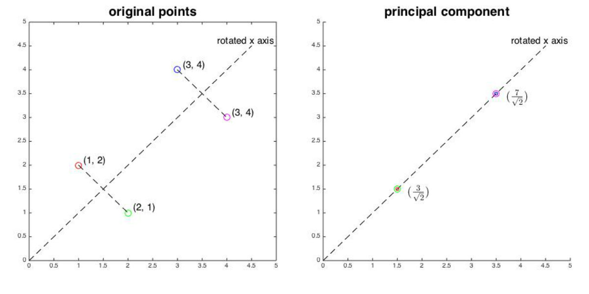
When we apply PCA algorithm on a data matrix $\mathbf{M} \in \mathbb{R}^{n \times d}$ , we actually project each data point $\mathbf{x}^{(i)} \in \mathbb{R}^d$ onto another space $\mathbb{R}^k$ , where $k < d$ . The $\mathbb{R}^k$ space, called the principal subspace, is where the variance of the projected data points (also called the principal components) is maximized. In other words, when the original data points are transformed into the principal subspace, they are most “spread out”. For example, suppose that there is a collection of four $\mathbb{R}^2$ data points $\{(1,2), (2,1), (3,4), (4,3)\}$ , we can obtain the raw data matrix:

$\mathbf{M} = \begin{bmatrix} 1 & 2 \\ 2 & 1 \\ 3 & 4 \\ 4 & 3 \end{bmatrix}$

Next, we compute $\mathbf{M}^\top\mathbf{M}$ and find its eigenpairs:

$\lambda_1 = 58, ~ \mathbf{v}_1 = \begin{bmatrix} \frac{1}{\sqrt{2}} \\ \frac{1}{\sqrt{2}} \end{bmatrix}, ~~~ \lambda_2 = 2, ~ \mathbf{v}_2 = \begin{bmatrix} \frac{1}{\sqrt{2}} \\ -\frac{1}{\sqrt{2}} \end{bmatrix}$

Now we want to compress the matrix $\mathbf{M}$ . Here, we can only set $k = 1$ and transform each data point into $\mathbb{R}$ space. Therefore, we multiply $\mathbf{M}$ by the principal eigenvector $\mathbf{v}_1$ and obtain:

$\mathbf{Mv}_1 = \begin{bmatrix} 1 & 2 \\ 2 & 1 \\ 3 & 4 \\ 4 & 3 \end{bmatrix} \times \begin{bmatrix} \frac{1}{\sqrt{2}} \\ \frac{1}{\sqrt{2}} \end{bmatrix} = \begin{bmatrix} 1 \times \frac{1}{\sqrt{2}} + 2 \times \frac{1}{\sqrt{2}} \\ 2 \times \frac{1}{\sqrt{2}} + 1 \times \frac{1}{\sqrt{2}} \\ 3 \times \frac{1}{\sqrt{2}} + 4 \times \frac{1}{\sqrt{2}} \\ 4 \times \frac{1}{\sqrt{2}} + 3 \times \frac{1}{\sqrt{2}} \end{bmatrix} = \begin{bmatrix} \frac{3}{\sqrt{2}} \\ \frac{3}{\sqrt{2}} \\ \frac{7}{\sqrt{2}} \\ \frac{7}{\sqrt{2}} \end{bmatrix}$

Note that each element of the principal component is the linear combination of all the elements of the original data point. Hence, the principal components retain most of information of original data points, while discarding some unimportant information such as noise. For original data points in $\mathbb{R}^2$ , the variances of the two dimensions are:

$\text{Var}_1 = \frac{1}{4} \times \big[(1-2.5)^2+(2-2.5)^2+(3-2.5)^2+(4-2.5)^2\big] = 1.25 \\ \text{Var}_2 = \frac{1}{4} \times \big[(2-2.5)^2+(1-2.5)^2+(4-2.5)^2+(3-2.5)^2\big] = 1.25$

For projected data point in the principal subspace, the variance is:

$\text{Var}_p = \frac{1}{4} \times \big[(\frac{3}{\sqrt{2}}-\frac{5}{\sqrt{2}})^2+(\frac{3}{\sqrt{2}}-\frac{5}{\sqrt{2}})^2+(\frac{7}{\sqrt{2}}-\frac{5}{\sqrt{2}})^2+(\frac{7}{\sqrt{2}}-\frac{5}{\sqrt{2}})^2\big] = 2.0$

We can find that the variance of the first dimension of the principal component is larger than any dimension of the original points, which demonstrates that PCA represents each data point on an axis, along which the variance of the data is maximized. As the following $\text{Figure}~ 1$ shows, the eigen matrix $E = \begin{bmatrix} 1/\sqrt{2} & -1/\sqrt{2} \\ 1/\sqrt{2} & 1/\sqrt{2} \end{bmatrix}$ can be viewed as a rotation 45 degrees counterclockwise of the axes. When we project each data point onto the rotated $x$ axis, we can see that they are most “spread out”.

$\text{Figure 1: PCA Transformation}$

In PCA, we project original data points onto $k$ axes corresponding to $k$ largest eigenvalues. Such $k$ axes store the raw data with maximized variances and thus retain most of information about original data. Therefore, we can concentrate on analyzing these principal components without worrying about the loss of unimportant information.

Using Covariance Matrix to Develop PCA

Knowing that PCA helps to maximize the variance of data points gives us another way to derive the algorithm, that is, computing the eigenpairs of the covariance matrix of the raw data. Suppose that there is a data matrix containing $n$ data points $\mathbf{M}=[\mathbf{x}^{(1)}; \mathbf{x}^{(2)}; ...; \mathbf{x}^{(n)}] \in \mathbb{R}^{n \times d}$ . We want to compress the raw data into $\mathbb{R}^k$ space. For simplicity, we set $k = 1$ , which means the principal component of each data point after transformation is a scalar value. Since the transformed scalar is the linear combination of all the elements of the original data point, there must be a vector $\mathbf{u} \in \mathbb{R}^d$ to complete the transformation:

$v^{(i)} = \mathbf{u}^\top \mathbf{x}^{(i)}, ~~i = 1, 2, ..., n$

Without loss of generality, $\mathbf{u}$ should be a unit vector such that $\mathbf{u}^\top\mathbf{u} = 1$ . And we finally compress the data matrix $\mathbf{M}$ into $\mathbf{v} = \mathbf{Mu} \in \mathbb{R}^n$ . And the unbiased variance of all points after projection is:

$\sigma^2 = \frac{1}{n-1} \sum_{i=1}^n \big[v^{(i)} - \mathbb{E}(v)\big]^2 \\ \mathbb{E}(v) = \frac{1}{n} \sum_{i=1}^n v^{(i)} = \frac{1}{n} \sum_{i=1}^n \mathbf{u}^\top \mathbf{x}^{(i)} = \mathbf{u}^\top \frac{1}{n}\sum_{i=1}^n \mathbf{x}^{(i)} = \mathbf{u}^\top \mathbb{E}(\mathbf{x})$

Substituting $v^{(i)}$ and $\mathbb{E}(v)$ we obtain:

$\sigma^2 = \frac{1}{n-1} \sum_{i=1}^n \big[\mathbf{u}^\top \mathbf{x}^{(i)} - \mathbf{u}^\top \mathbb{E}(\mathbf{x})\big]^2 = \mathbf{u}^\top \mathbf{S} \mathbf{u}$

where $\mathbf{S}$ is the data covariance matrix:

$\mathbf{S} = \frac{1}{n-1}\sum_{i=1}^n \big[\mathbf{x}^{(i)} - \mathbb{E}(\mathbf{x})\big] \big[\mathbf{x}^{(i)} - \mathbb{E}(\mathbf{x})\big]^\top = \begin{bmatrix} \text{Var}(\mathbf{x}_1) & \text{Cov}(\mathbf{x}_1, \mathbf{x}_2) & \cdots & \text{Cov}(\mathbf{x}_1, \mathbf{x}_n) \\ \text{Cov}(\mathbf{x}_2, \mathbf{x}_1) & \text{Var}(\mathbf{x}_2) & \cdots & \text{Cov}(\mathbf{x}_2, \mathbf{x}_n) \\ \vdots & \vdots & \ddots & \vdots \\ \text{Cov}(\mathbf{x}_n, \mathbf{x}_1) & \text{Cov}(\mathbf{x}_n, \mathbf{x}_2) & \cdots & \text{Var}(\mathbf{x}_n) \end{bmatrix} = \frac{1}{n-1} \mathbf{X}^\top\mathbf{X}$

where $\text{Var}(\mathbf{x}_i)$ denotes the variance of the $i$ -th dimension of the original data points, $\text{Cov}(\mathbf{x}_i, \mathbf{x}_j)$ denotes the covariance between $i$ -th and $j$ -th dimensions and $\mathbf{X} = [\mathbf{x}^{(1)} - \mathbb{E}(\mathbf{x}); \mathbf{x}^{(2)} - \mathbb{E}(\mathbf{x}); ...; \mathbf{x}^{(n)} - \mathbb{E}(\mathbf{x})] \in \mathbb{R}^{n \times d}$ . Since PCA maximizes the variance of original data points, we now maximize the projected variance:

$\mathop{\arg\max}_{\mathbf{u}}\mathbf{u}^\top\mathbf{Su} ~~~~s.t.~~ \mathbf{u}^\top\mathbf{u} = 1$

The Rayleigh–Ritz theorem tells us the solution to the optimization problem above is the principal eigenvector (the eigenvector corresponds to the largest eigenvalue) of the covariance matrix $\mathbf{S}$ .

Finally, we can eigendecompose the covariance matrix $\mathbf{S}$ of the raw data matrix $\mathbf{M}$ and find the $k$ principal eigenvectors to compress the original data. It works similarily to the eigendecomposition of matrix $\mathbf{M}^\top\mathbf{M}$ but not exactly the same, since the principal eigenvectors of $\mathbf{M}^\top\mathbf{M}$ and $\mathbf{S}$ may not be the same. Considering our previous example:

import numpy as np

M = np.array([[1,2], [2,1], [3,4], [4,3]])
Cov = np.cov(M.T)  # Compute the covariance matrix of M

lams_1, vecs_1 = np.linalg.eig(np.dot(M.T, M))  # Eigendecompose M'M
lams_2, vecs_2 = np.linalg.eig(Cov)             # Eigendecompose the covariance matrix
print("original data matrix:")
print(M)
print("eigenvalues of M'M:", lams_1)
print("eigenvalues of Cov:", lams_2)

# get the unique eigenvectors
for i in range(vecs_1.shape[1]):
    if vecs_1[0, i] < 0: vecs_1[:, i] = vecs_1[:, i] * -1
for i in range(vecs_2.shape[1]):
    if vecs_2[0, i] < 0: vecs_2[:, i] = vecs_2[:, i] * -1

print("eigenvectors of M'M: ")
print(vecs_1)
print("eigenvectors of Cov: ")
print(vecs_2)
print("The compressed M by eigendecomposing M'M:", np.dot(M, vecs_1[:, 0]))
print("The compressed M by eigendecomposing Cov:", np.dot(M, vecs_2[:, 0]))

original data matrix:
[[1 2]
 [2 1]
 [3 4]
 [4 3]]
eigenvalues of M'M: [58.  2.]
eigenvalues of Cov: [2.66666667 0.66666667]
eigenvectors of M'M: 
[[ 0.70710678  0.70710678]
 [ 0.70710678 -0.70710678]]
eigenvectors of Cov: 
[[ 0.70710678  0.70710678]
 [ 0.70710678 -0.70710678]]
The compressed M by eigendecomposing M'M: [2.12132034 2.12132034 4.94974747 4.94974747]
The compressed M by eigendecomposing Cov: [2.12132034 2.12132034 4.94974747 4.94974747]

Here we got the same eigenvectors but different eigenvalues by eigendecomposing $\mathbf{M}^\top\mathbf{M}$ and $\mathbf{S}$ , respectively. Therefore, the two methods obtain the same compressed data. Under situations where the two methods get different eigenvectors, we might obtain different compressed data:

M = np.random.rand(4,2) * 4
Cov = np.cov(M.T)  # Compute the covariance matrix of M

lams_1, vecs_1 = np.linalg.eig(np.dot(M.T, M))  # Eigendecompose M'M
lams_2, vecs_2 = np.linalg.eig(Cov)             # Eigendecompose the covariance matrix
print("original data matrix:")
print(M)
print("eigenvalues of M'M:", lams_1)
print("eigenvalues of Cov:", lams_2)

# get the unique eigenvectors
for i in range(vecs_1.shape[1]):
    if vecs_1[0, i] < 0: vecs_1[:, i] = vecs_1[:, i] * -1
for i in range(vecs_2.shape[1]):
    if vecs_2[0, i] < 0: vecs_2[:, i] = vecs_2[:, i] * -1

print("eigenvectors of M'M: ")
print(vecs_1)
print("eigenvectors of Cov: ")
print(vecs_2)
print("The compressed M by eigendecomposing M'M:", np.dot(M, vecs_1[:, 0]))
print("The compressed M by eigendecomposing Cov:", np.dot(M, vecs_2[:, 0]))

original data matrix:
[[2.84662895 0.72347183]
 [1.2427886  1.44384041]
 [0.9416138  3.39384996]
 [3.2100749  1.21335165]]
eigenvalues of M'M: [29.47256331  6.96500039]
eigenvalues of Cov: [0.32558503 2.33611369]
eigenvectors of M'M: 
[[ 0.78512207  0.61934105]
 [ 0.61934105 -0.78512207]]
eigenvectors of Cov: 
[[ 0.72246974  0.69140254]
 [ 0.69140254 -0.72246974]]
The compressed M by eigendecomposing M'M: [2.68302702 1.8699704  2.84123236 3.27177914]
The compressed M by eigendecomposing Cov: [2.55681353 1.89615209 3.02680397 3.15809639]

Usually, we prefer to directly use the covariance matrix $\mathbf{S}$ to develop the PCA algorithm since it ensures that the variances of original data points are maximized.

Using Correlation Matrix to Develop PCA

Sometimes the variances of the dimensions in our data are significantly different. In this case, we need to scale the data to unit variance. In other hands, let $\mathbb{E}(\mathbf{x}) = [\mathbb{E}(\mathbf{x}_1); \mathbb{E}(\mathbf{x}_2); ...; \mathbb{E}(\mathbf{x}_d)]$ and $\text{Var}(\mathbf{x}) = [\text{Var}(\mathbf{x}_1); \text{Var}(\mathbf{x}_2); ...; \text{Var}(\mathbf{x}_d)]$ , we need to standardize the raw data points:

$\mathbf{x}^{'(i)} = \frac{\mathbf{x}^{(i)} - \mathbb{E}(\mathbf{x})}{\sqrt{\text{Var}(\mathbf{x})}}, ~~i=1,2,...,n$

And then we obtain the standard matrix $\mathbf{M}_s = [\mathbf{x}^{'(1)}; \mathbf{x}^{'(2)}; ...; \mathbf{x}^{'(n)}]$ . Next, we compute the correlation matrix of the original matrix $\mathbf{M}$ :

$\mathbf{C} = \frac{1}{n} \mathbf{M}_s^\top \mathbf{M}_s$

Finally, we use principal eigenvectors of the correlation matrix $\mathbf{C}$ to develop the PCA.

The compressed data obtained by eigendecomposing covariance and correlation matrices is usually different. This is mainly because the process of standardizing raw data to gain correlation matrix is actually reducing the differences between the variances of different dimensions in original data. Which matrix to choose depends on the demands of the environmental settings.

Reduce Computational Complexity

Similar to the eigendecomposition of $\mathbf{M}^\top\mathbf{M}$ , when the situation $n << d$ comes, we can first compute the eigenpairs of $\mathbf{XX}^\top$ or $\mathbf{M}_s\mathbf{M}_s^\top$ and then obtain the eigenvectors of covariance or correlation matrix by multiplication $\mathbf{X}^\top \mathbf{e}$ or $\mathbf{M}_s^\top \mathbf{e}$ , where $\mathbf{e}$ is the eigenvector of matrix $\mathbf{XX}^\top$ or $\mathbf{M}_s\mathbf{M}_s^\top$ . This operation can effectively reduce the computation complexity. See our last blog for details.

More Complete PCA Algorithm

Given a set of data sample $\mathcal{X}=\{\mathbf{x}^{(1)}, \mathbf{x}^{(2)}, ..., \mathbf{x}^{(n)}\}$ , create the raw data matrix $\mathbf{M} = [\mathbf{x}^{(1)}; \mathbf{x}^{(2)}; ...; \mathbf{x}^{(n)}]$ or the standard matrix $\mathbf{M}_s = [\frac{\mathbf{x}^{(1)} - \mathbb{E}(\mathbf{x})}{\sqrt{\text{Var}(\mathbf{x})}}; \frac{\mathbf{x}^{(2)} - \mathbb{E}(\mathbf{x})}{\sqrt{\text{Var}(\mathbf{x})}}; ...; \frac{\mathbf{x}^{(n)} - \mathbb{E}(\mathbf{x})}{\sqrt{\text{Var}(\mathbf{x})}}]$ .
Compute all eigenpairs of the symmetric matrix $\mathbf{M}^\top\mathbf{M}$ or the corvariance matrix $\mathbf{X}^\top\mathbf{X}$ or the corelation matrix $\mathbf{M}^\top_s\mathbf{M}_s$ . When the number of columns are much larger than the number of rows, we compute the eigenpairs of $\mathbf{MM}^\top$ or $\mathbf{XX}^\top$ or $\mathbf{M}_s\mathbf{M}_s^\top$ and use them to find the $k$ largest eigenpairs we need.
Use $k$ eigenvectors corresponding to $k$ largest eigenvalues as columns to form the eigenmatrix $\mathbf{D}$ .
Apply matrix multiplication $\mathbf{M}^{'}=\mathbf{MD}$ to compress the raw data.
Use $\mathbf{M}^{r} = \mathbf{M}^{'}\mathbf{D}^\top \approx \mathbf{M}$ to approximately reconstruct the raw data when necessary.

Conclusion

In this blog, we open the black box of the PCA and develop a more complete algorithm. We hope this blog can help understand the PCA algorithm more deeply.

Principal Component Analysis (II)

Open the black box of PCA algorithm