Quadratic Optimization

Introduction

Quadratic optimization problems appear frequently in the fields of engineering and computer science. Lots of problems in the real world can be expressed as the minimization or maxmization of some energy/cost function, with or without constraints. And the simplest kind of such a function is a quadratic function. This blog introduces the matrix forms of pure quadratic equations and two common quadratic optimization problems.

Quadratic Equation and Symmetric Matrix

A pure quadratic equation, that is, an equation with only quadratic terms, can be expressed as:

$\mathrm{a}x^2 + 2\mathrm{b}xy + \mathrm{c}y^2 = \mathrm{C}$

where $x, y$ are variables, $\mathrm{a, b, c}$ are constant coefficients and $\mathrm{C}$ is a constant. Denote the vector $\mathbf{x}=\begin{bmatrix} x \\ y \end{bmatrix}$ and the symmetric matrix $\mathbf{M}=\begin{bmatrix} \mathrm{a} & \mathrm{b} \\ \mathrm{b} & \mathrm{c} \end{bmatrix}$ . Then we can restate the quadratic equation above as the matrix multiplication:

$\mathrm{a}x^2 + 2\mathrm{b}xy + \mathrm{c}y^2 = \mathrm{C} \Leftrightarrow \begin{bmatrix} x & y \end{bmatrix} \begin{bmatrix} \mathrm{a} & \mathrm{b} \\ \mathrm{b} & \mathrm{c} \end{bmatrix} \begin{bmatrix} x \\ y \end{bmatrix} = \mathbf{x}^\top\mathbf{Mx} = \mathrm{C}$

Similarly, pure quadratic expressions with multiple variables can also be represented as corresponding matrix forms:

$\begin{align} \mathrm{a}x^2 + \mathrm{e}y^2 + \mathrm{f}z^2 + 2\mathrm{b}xy + 2\mathrm{c}xz + 2\mathrm{d}yz &= \mathrm{C} \Leftrightarrow \begin{bmatrix} x & y & z \end{bmatrix} \begin{bmatrix} \mathrm{a} & \mathrm{b} & \mathrm{c} \\ \mathrm{b} & \mathrm{e} & \mathrm{d} \\ \mathrm{c} & \mathrm{d} & \mathrm{f} \end{bmatrix} \begin{bmatrix} x \\ y \\ z \end{bmatrix} = \mathrm{C} \\ \begin{matrix} \mathrm{a} x^2 + \mathrm{l} y^2 + \mathrm{m} z^2 + \mathrm{n} u^2 + \mathrm{p} v^2 + 2\mathrm{b} xy + 2\mathrm{c} xz + 2\mathrm{d} xu \\ + 2\mathrm{e} xv + 2\mathrm{f}yz + 2\mathrm{g} yu + 2\mathrm{h} yv + 2\mathrm{i} zu + 2\mathrm{j} zv + 2\mathrm{k}uv \end{matrix} &= \mathrm{C} \Leftrightarrow \begin{bmatrix} x & y & z & u & v \end{bmatrix} \begin{bmatrix} \mathrm{a} & \mathrm{b} & \mathrm{c} & \mathrm{d} & \mathrm{e} \\ \mathrm{b} & \mathrm{l} & \mathrm{f} & \mathrm{g} & \mathrm{h} \\ \mathrm{c} & \mathrm{f} & \mathrm{m} & \mathrm{i} & \mathrm{j} \\ \mathrm{d} & \mathrm{g} & \mathrm{i} & \mathrm{n} & \mathrm{k} \\ \mathrm{e} & \mathrm{h} & \mathrm{j} & \mathrm{k} & \mathrm{p} \\ \end{bmatrix} \begin{bmatrix} x \\ y \\ z \\ u \\ v \end{bmatrix} = \mathrm{C} \end{align}$

Quadratic Function and Eigenvectors

Usually, we are interested in estimating the value of a quadratic function with or without constraints:

$f(\mathbf{x}) = \mathbf{x}^\top \mathbf{Mx}$

In this case, the eigenvectors of the symmetric matrix $\mathbf{M}$ tells us the information about the gradient direction of the function $f(\mathbf{x})$ . For example, suppose that $\mathbf{x} = \begin{bmatrix} x_1 \\ x_2 \end{bmatrix} \in \mathbb{R}^2$ and $\mathbf{M}=\begin{bmatrix} 3 & 2 \\ 2 & 6 \end{bmatrix}$ , we first compute the eigenvectors and eigenvalues of the matrix $\mathbf{M}$ (Methods for computing eigenpairs are discussed in this blog):

$\mathbf{v}^{(1)} = \begin{bmatrix} 0.4472 \\ 0.8944 \end{bmatrix}, \lambda_1 = 7.0 ~~~~ \mathbf{v}^{(2)} = \begin{bmatrix} 0.8944 \\ -0.4472 \end{bmatrix}, \lambda_2 = 2.0$

Next, we draw the contour map of the function $f(\mathbf{x})$ and mark the directions of the two eigenvectors:

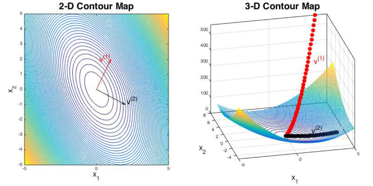
$\text{Figure 1: Directions of eigenvectors}$

We can see that the direction of the eigenvector with largest eigenvalue ( $\mathbf{v}^{(1)}$ ) indicates the steepest gradient direction of $f(\mathbf{x})$ while the eigenvector with smallest eigenvalue ( $\mathbf{v}^{(2)}$ ) indicates the most gradual gradient direction. In other words, the quadratic function $f(\mathbf{x})$ changes fastest along the direction of $\mathbf{v}^{(1)}$ while changes slowest along the direction of $\mathbf{v}^{(2)}$ .

Quadratic Optimization Problems

In this section, we introduce two common quadratic optimization problems and their corresponding theories.

Rayleigh–Ritz Ratio

For the following quadratic problems:

$\begin{align} f_1(\mathbf{x}) &= \max_{\mathbf{x}} \mathbf{x}^\top \mathbf{Mx} ~~s.t.~~ \lvert\lvert\mathbf{x}\rvert\rvert = 1 \\ f_2(\mathbf{x}) &= \min_{\mathbf{x}} \mathbf{x}^\top \mathbf{Mx} ~~s.t.~~ \lvert\lvert\mathbf{x}\rvert\rvert = 1 \end{align}$

where $\mathbf{x} \in \mathbb{R}^n$ and $\mathbf{M} \in \mathbb{R}^{n \times n}$ , we can find the solution according to the Rayleigh–Ritz theorem:

$\begin{align} &\text{If $\mathbf{M}$ is a symmetric $n \times n$ matrix with eigenvalues $\lambda_1 \ge \lambda_2 \ge ... \ge \lambda_n$ and if $\{\mathbf{v}_1, ..., \mathbf{v}_n\}$ is any} \\ &\text{orthogonal eigenvector set of $\mathbf{M}$, where $\mathbf{v}_i$ is an eigenvector associated with $\lambda_i$, then} \end{align}$ $\max \frac{\mathbf{x}^\top \mathbf{Mx}}{\mathbf{x}^\top \mathbf{x}} = \lambda_1 ~~\text{with}~~ \mathbf{x}=\mathbf{v}_1 \\ \min \frac{\mathbf{x}^\top \mathbf{Mx}}{\mathbf{x}^\top \mathbf{x}} = \lambda_n ~~\text{with}~~ \mathbf{x}=\mathbf{v}_n$

The ratio $\frac{\mathbf{x}^\top \mathbf{Mx}}{\mathbf{x}^\top \mathbf{x}}$ is known as the Rayleigh–Ritz ratio. When $\lvert\lvert\mathbf{x}\rvert\rvert = 1$ , we have $\mathbf{x}^\top \mathbf{x} = 1$ , and we can normalize each $\mathbf{v}_i$ into a unit eigenvector $\mathbf{v}_i^{'}$ and obtain the optimized solution:

$\begin{align} f_1(\mathbf{x}) &= \max \mathbf{x}^\top \mathbf{Mx} = \lambda_1 ~~\text{with}~~ \mathbf{x}=\mathbf{v}_1^{'} \\ f_2(\mathbf{x}) &= \min \mathbf{x}^\top \mathbf{Mx} = \lambda_n ~~\text{with}~~ \mathbf{x}=\mathbf{v}_n^{'} \end{align}$

This conclusion is essential for the Principle Component Analysis (PCA) algorithm, as we will see in my later blogs. In addition, we can derive a corollary from the Rayleigh–Ritz theorem:

$\begin{align} & \text{If } \mathbf{x} \in \{\mathbf{v}^{(1)}, \mathbf{v}^{(2)}, ..., \mathbf{v}^{(j-1)}\}^\perp,~~ \text{ then } \max \frac{\mathbf{x}^\top \mathbf{Mx}}{\mathbf{x}^\top \mathbf{x}} = \lambda_j \text{ with } \mathbf{x} = \mathbf{v}^{(j)} \\ & \text{If } \mathbf{x} \in \{\mathbf{v}^{(j+1)}, \mathbf{v}^{(j+2)}, ..., \mathbf{v}^{(n)}\}^\perp,~~ \text{ then } \min \frac{\mathbf{x}^\top \mathbf{Mx}}{\mathbf{x}^\top \mathbf{x}} = \lambda_j \text{ with } \mathbf{x} = \mathbf{v}^{(j)} \end{align}$

where $\perp$ denotes the orthogonal complement.

Positive Definite Quadratic Function

Another common quadratic optimization problem is:

$f(\mathbf{x}) = \min_{\mathbf{x}} \frac{1}{2} \mathbf{x}^\top \mathbf{Mx} + \mathbf{x}^\top \mathbf{b}$

where $\mathbf{x} \in \mathbb{R}^n$ and $\mathbf{M} \in \mathbb{R}^{n \times n}$ . If $\mathbf{M}$ is a positive definite symmetric matrix, we can obtain the optimized solution through the following proposition:

$\text{If $\mathbf{M}$ is symmetric positive definite, then } \\ P(\mathbf{x}) = \frac{1}{2} \mathbf{x}^\top \mathbf{Mx} + \mathbf{x}^\top \mathbf{b} \\ \text{assumes its minimum at the point $\mathbf{Mx} = \mathbf{b}$.}$

In order to prove the proposition above, the first thing we need to know is that $\forall \mathbf{x}, \mathbf{x}^\top \mathbf{Mx} > 0$ if $\mathbf{M}$ is symmetric, which can be easily proved by Rayleigh–Ritz theorem. Then we can prove the proposition above:

$Proof. ~~\text{Let $\mathbf{x}$ be the solution of $\mathbf{Mx} = \mathbf{b}$. Then, $\forall \mathbf{y} \in \mathbb{R}^n$ and $\mathbf{y} \ne \mathbf{x}$}, \\ \begin{align} P(\mathbf{y}) - P(\mathbf{x}) &= \big(\frac{1}{2} \mathbf{y}^\top \mathbf{My} - \mathbf{y}^\top \mathbf{b} \big) - \big(\frac{1}{2} \mathbf{x}^\top \mathbf{Mx} - \mathbf{x}^\top \mathbf{b} \big) \\ &= \big(\frac{1}{2} \mathbf{y}^\top \mathbf{My} - \mathbf{y}^\top \mathbf{b} \big) - \big(\frac{1}{2} \mathbf{x}^\top \mathbf{Mx} - \mathbf{x}^\top \mathbf{Mx} \big) \\ &= \big(\frac{1}{2} \mathbf{y}^\top \mathbf{My} - \mathbf{y}^\top \mathbf{Mx} \big) - \big(-\frac{1}{2} \mathbf{x}^\top \mathbf{Mx}\big) \\ &= \frac{1}{2} \mathbf{y}^\top \mathbf{My} - \mathbf{y}^\top \mathbf{Mx} + \frac{1}{2} \mathbf{x}^\top \mathbf{Mx} \\ &= \frac{1}{2} \mathbf{y}^\top \mathbf{My} - \frac{1}{2} \mathbf{y}^\top \mathbf{Mx} - \frac{1}{2} \mathbf{y}^\top \mathbf{Mx} + \frac{1}{2} \mathbf{x}^\top \mathbf{Mx} \\ &= \frac{1}{2} \mathbf{y}^\top \mathbf{My} - \frac{1}{2} \mathbf{y}^\top \mathbf{Mx} - \frac{1}{2} \mathbf{x}^\top \mathbf{My} + \frac{1}{2} \mathbf{x}^\top \mathbf{Mx} \\ &= \frac{1}{2} (\mathbf{y}-\mathbf{x})^\top \mathbf{M} (\mathbf{y} - \mathbf{x}) > 0 \end{align}$

Note that $\mathbf{y}^\top \mathbf{Mx} = \mathbf{x}^\top \mathbf{My}$ since $\mathbf{M}$ is symmetric. Hence, the optimized solution of $f(\mathbf{x})$ is the solution of $\mathbf{Mx} = \mathbf{b}$ .

Conclusion

In this blog, we introduce the concept of quadratic optimization problems, the relationship between quadratic function and symmetric matrix and two common quadratic optimization problems with their solutions.

Quadratic Optimization

Introduce common quadratic optimization problems