Eigendecomposition

Introduction

Eigendecomposition of a matrix, in which we decompose the matrix into a set of eigenvectors and eigenvalues, shows us to the information about the universal and functional properties of the matrix. Such properties might not be obvious from the representation of the matrix as an array of elements. This blog introduces the related concepts of matrix eigendecomposition and methods to compute eigenvectors and eigenvalues of a matrix.

Eigenvalue and Eigenvector

An eigenvector of a square matrix $\mathbf{A}$ is a nonzero vector $\mathbf{v}$ such that multiplication by $\mathbf{A}$ alters only the scale of $\mathbf{v}$ : $\mathbf{Av} = \lambda \mathbf{v}$ . Where $\lambda$ is the eigenvalue corresponding to the eigenvector $\mathbf{v}$ .

Note that if $\mathbf{v}$ is the eigenvector of $\mathbf{A}$ , then $s\mathbf{v}~(s \in \mathbb{R}, s \ne 0)$ is also the eigenvector of $\mathbf{A}$ with the same eigenvalue $\lambda$ . Therefore, we usually focus on the unit eigenvectors, which means $\lvert\lvert\mathbf{v}\rvert\rvert = 1$ . Even that is not quite enough to make the eigenvector unique, since we may still multiply it by $-1$ to obtain another eigenvector with the same eigenvalue. Hence, we shall also require that the first nonzero component of an eigenvector be positive.

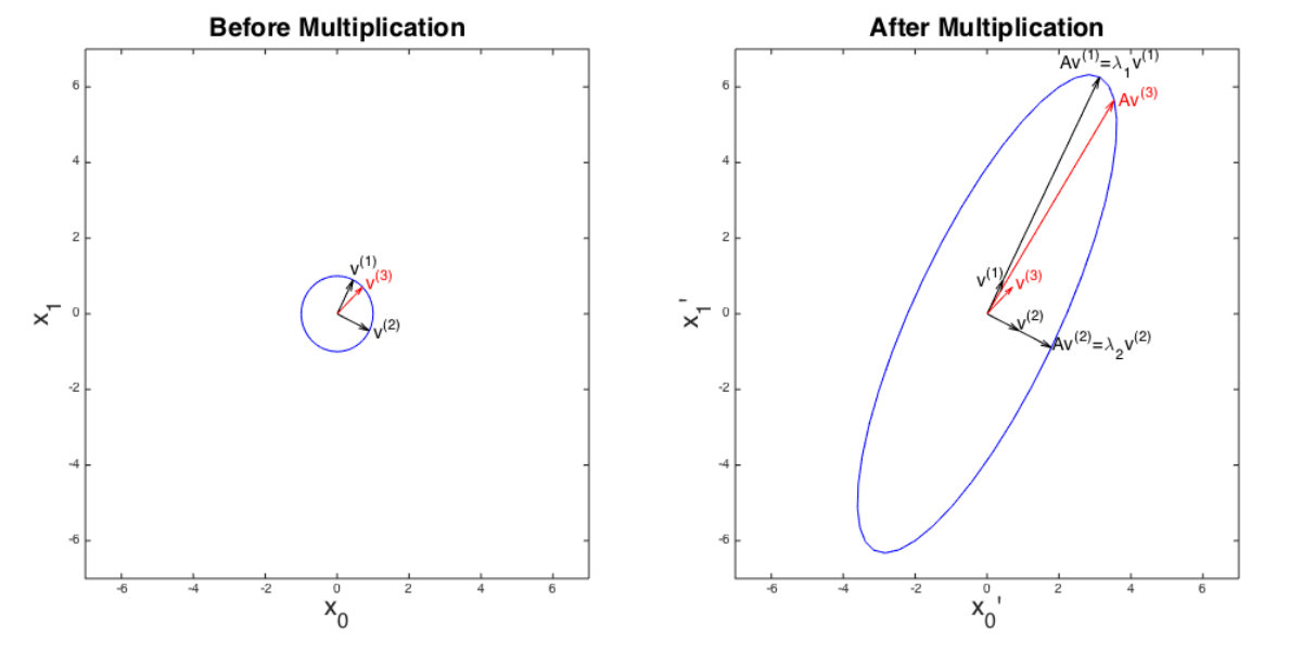
Intuitively, the multiplication $\mathbf{Av}$ maps the vector $\mathbf{v}$ into another space, probably changing its size, direction or dimension. Particularly, if $\mathbf{v}$ is the eigenvector of $\mathbf{A}$ , $\mathbf{Av}$ only scale $\mathbf{v}$ by corresponding eigenvalue $\lambda$ . $\text{Figure 1}$ shows the differences between the transformations of eigenvectors and non-eigenvectors. For eigenvectors $\mathbf{v}^{(1)}$ and $\mathbf{v}^{(2)}$ of $\mathbf{A}$ , the multiplication only changes their size. For non-eigenvectors $\mathbf{v}^{(3)}$ , the multiplication not only changes its size but also its direction.

$\text{Figure 1: Vector Transformations}$

For an $n \times n$ square matrix, there will always be $n$ eigenpairs (an eigenvalue and its corresponding eigenvector), although in some cases, some of the eigenvalues will be identical. And the eigenvector with the largest eigenvalue is called the principal eigenvector.

Computing Eigenvalues and Eigenvectors

There are various algorithms to compute eigenpairs of a matrix. Here we introduce two general methods.

Determinant

The determinant of a square matrix $\mathbf{A}$ , denoted as $det(\mathbf{A})$ or $\lvert\mathbf{A}\rvert$ , is a function that maps matrices to real scalars. According to the rule that the determinant of a matrix $\mathbf{M}$ must be 0 in order for $\mathbf{Mx} = \mathbf{0}$ to hold for a vector $\mathbf{x} \ne 0$ , we can develop a basic method to compute eigenpairs for the matrix $\mathbf{M}$ .

We first restate the equation $\mathbf{Av} = \lambda \mathbf{v}$ as $(\mathbf{A}-\lambda \mathbf{I})\mathbf{v} = \mathbf{0}$ . The eigenvector $\mathbf{v}$ must be nonzero and thus the determinent of $\mathbf{A}-\lambda \mathbf{I}$ must be 0. The determinant of $\mathbf{A}-\lambda \mathbf{I}$ is an $n$ -th degree polynomial in $\lambda$ , whose roots are $n$ eigenvectors of the matrix $\mathbf{A}$ . For each eigenvalue $\lambda_i$ , we can obtain a vector $\mathbf{v}^{(i)}$ by solving the equation $\mathbf{Av}^{(i)} = \lambda_i \mathbf{v}^{(i)}$ . Finally, we normalize $\mathbf{v}^{(i)}$ to get the eigenvector corresponding to the eigenvalue $\lambda_i$ . For example, consider the matrix:

$\mathbf{A} = \begin{bmatrix} -2 & -2 & 4 \\ -2 & 1 & 2 \\ 4 & 2 & 5 \end{bmatrix}$

Then $\mathbf{A}-\lambda \mathbf{I}$ is:

$\mathbf{A}-\lambda \mathbf{I} = \begin{bmatrix} -2-\lambda & -2 & 4 \\ -2 & 1-\lambda & 2 \\ 4 & 2 & 5-\lambda \end{bmatrix}$

Considering the first row as the referenced row, we obtain the determinent equation:

$(-2-\lambda)\begin{vmatrix} 1-\lambda & 2 \\ 2 & 5-\lambda \end{vmatrix} + 2 \begin{vmatrix} -2 & 2 \\ 4 & 5-\lambda \end{vmatrix} + 4 \begin{vmatrix} -2 & 1-\lambda \\ 4 & 2 \end{vmatrix} = 0 \\ (-2-\lambda)\big[(1-\lambda)(5-\lambda) - 2 \times 2\big]+2\big[(-2)(5-\lambda)-4\times2\big]+4\big[-2 \times 2 - 4(1-\lambda)\big] = 0 \\ - \lambda^3 + 4 \lambda^2 + 31 \lambda - 70 = 0$

By trial and error, we factor the equation into:

$(\lambda-2)(\lambda+5)(\lambda-7)=0$

Solving the equation gives three eigenvalues $\lambda_1 = 2$ , $\lambda_2 = -5$ and $\lambda_3=7$ . Then we use the eigenvalues to compute the corresponding eigenvectors:

$\begin{align} \mathbf{Av}^{(1)} = \lambda_1 \mathbf{v}^{(1)} \Rightarrow \begin{bmatrix} -2 & -2 & 4 \\ -2 & 1 & 2 \\ 4 & 2 & 5 \end{bmatrix} \begin{bmatrix} x_1 \\ y_1 \\ z_1 \end{bmatrix} &= 2 \begin{bmatrix} x_1 \\ y_1 \\ z_1 \end{bmatrix} \\ \mathbf{Av}^{(2)} = \lambda_2 \mathbf{v}^{(2)} \Rightarrow \begin{bmatrix} -2 & -2 & 4 \\ -2 & 1 & 2 \\ 4 & 2 & 5 \end{bmatrix} \begin{bmatrix} x_2 \\ y_2 \\ z_2 \end{bmatrix} &= -5 \begin{bmatrix} x_2 \\ y_2 \\ z_2 \end{bmatrix} \\ \mathbf{Av}^{(3)} = \lambda_3 \mathbf{v}^{(3)} \Rightarrow \begin{bmatrix} -2 & -2 & 4 \\ -2 & 1 & 2 \\ 4 & 2 & 5 \end{bmatrix} \begin{bmatrix} x_3 \\ y_3 \\ z_3 \end{bmatrix} &= 7 \begin{bmatrix} x_3 \\ y_3 \\ z_3 \end{bmatrix} \end{align}$

Solving the three linear systems above and scale the vector we get three possible eigenvectors:

$\mathbf{v}^{(1)} = \begin{bmatrix} 1 \\ -2 \\ 0 \end{bmatrix}, \mathbf{v}^{(2)} = \begin{bmatrix} 2 \\ 1 \\ -1 \end{bmatrix}, \mathbf{v}^{(3)} = \begin{bmatrix} 2 \\ 1 \\ 5 \end{bmatrix}$

Finally, we normalize the three vectors into unit vectors:

$\mathbf{v}^{(1)} = \begin{bmatrix} 1 / \sqrt{1^2+(-2)^2+0^2} \\ -2 / \sqrt{1^2+(-2)^2+0^2} \\ 0 / \sqrt{1^2+(-2)^2+0^2} \end{bmatrix} \approx \begin{bmatrix} 0.4472 \\ -0.8944 \\ 0 \end{bmatrix} \\ \mathbf{v}^{(2)} = \begin{bmatrix} 2 / \sqrt{2^2+1^2+(-1)^2} \\ 1 / \sqrt{2^2+1^2+(-1)^2} \\ -1 / \sqrt{2^2+1^2+(-1)^2} \end{bmatrix} \approx \begin{bmatrix} 0.8165 \\ 0.4082 \\ -0.4082 \end{bmatrix} \\ \mathbf{v}^{(3)} = \begin{bmatrix} 2 / \sqrt{2^2+1^2+5^2} \\ 1 / \sqrt{2^2+1^2+5^2} \\ 5 / \sqrt{2^2+1^2+5^2} \end{bmatrix} \approx \begin{bmatrix} 0.3651 \\ 0.1826 \\ 0.9129 \\ \end{bmatrix}$

The major drawback of solving the determinant polynomial is that it is extremely inefficient for large matrices. The determinant of an $n \times n$ matrix has $n!$ terms, implying $O(n!)$ time for computation. Fortunately, various $O(n^3)$ algorithms have been proposed to compute the determinant more efficiently, such as the Decomposition methods.

Power Iteration

Compute the First Eigenpair

Power iteration is generally used to find the eigenvector with the largest (in absolute value) eigenvalue of a diagonalizable matrix $\mathbf{M}$ . We start with any nonzero vector $\mathbf{x}_0$ and then iterate:

$\mathbf{x}_{k+1} = \frac{\mathbf{Mx}_k}{\lvert\lvert\mathbf{Mx}_k\rvert\rvert}$

We do the iteration until convergence, that is, $\lvert\lvert\mathbf{x}_k − \mathbf{x}_{k+1}\rvert\rvert$ is less than some small constant or we’ve reached the maximum iterations defined before. Let $\mathbf{x}_f$ be the final vector we obtained. Then $\mathbf{x}_f$ is approximately the eigenvector with greatest absolute eigenvalue of $\mathbf{M}$ . Note that $\mathbf{x}_f$ will be a unit vector and thus we can get the corresponding eigenvalue simply by computing $\lambda = \mathbf{x}_f^\top \mathbf{Mx}_f$ , since $\mathbf{Mx}_f = \lambda \mathbf{x}_f \Rightarrow \mathbf{x}_f^\top\mathbf{Mx}_f = \mathbf{x}_f^\top \lambda \mathbf{x}_f = \lambda \mathbf{x}_f^\top\mathbf{x}_f = \lambda$ .

Again, we set the maximum iterations = 100, x_0 = array([[1],[1],[1]]) and use the power iteration to compute the first eigenpair of the matrix $\mathbf{A}$ defined in the last section:

import numpy as np

A = np.array([[-2.,-2.,4.],[-2.,1.,2.],[4.,2.,5.]])
max_iter = 100
x_0 = np.array([[1.],[1.],[1.]])
x_f = None
for _ in range(max_iter):
    x_f = np.dot(A, x_0)            # x_f = Ax_0
    x_f_norm = np.linalg.norm(x_f)  # ||Ax_0||
    x_f = x_f / x_f_norm            # Ax_0 / ||Ax_0||
    x_0 = x_f

tmp = np.dot(A, x_f)
x_f_T = x_f.reshape(1, -1)
lamda = np.dot(x_f_T, tmp)


print('First eigenvector of A:')
print(x_f)
print('First eigenvalue of A:', lamda[0][0])

First eigenvector of A:
[[0.36514837]
 [0.18257419]
 [0.91287093]]
First eigenvalue of A: 7.000000000000001

We see that power iteration yields the eigenpair that approximates the eigenpair with largest absolute eigenvalue obtained by solving the determinant polynomial. However, power iteration only computes the first eigenpair rather than all eigenpairs of a matrix. Fortunately, we can find all eigenpairs of a symmetric matrix by applying power iteration multiple times.

Find all Eigenpairs of Symmetric Matrix

For the symmetric matrix $\mathbf{A}$ defined in the last section, we first compute the first eigenvector of the original matrix. And then we remove the first eigenvector from $\mathbf{A}$ and obtain a modified matrix $\mathbf{B}$ . The first eigenvector of the new matrix $\mathbf{B}$ is the second eigenvector (eigenvector with the second-largest eigenvalue in absolute value) of the original matrix $\mathbf{A}$ . We continue this process until we find the last eigenvector. In each step of the process, power iteration is used to find the first eigenpair of the new matrix.

In the first step, we use power iteration to compute the first eigenpair of the original matrix $\mathbf{A}$ :

$\mathbf{v}^{(3)} \approx \begin{bmatrix} 0.3651 \\ 0.1826 \\ 0.9129 \\ \end{bmatrix}, \lambda_3 = 7.0$

In the second step, we create a new matrix

$\begin{align} \mathbf{B} = \mathbf{A} - \lambda_3 \mathbf{v}^{(3)} \mathbf{v}^{(3) \top} &= \begin{bmatrix} -2 & -2 & 4 \\ -2 & 1 & 2 \\ 4 & 2 & 5 \end{bmatrix} - 7.0 \times \begin{bmatrix} 0.3651 \\ 0.1826 \\ 0.9129 \\ \end{bmatrix} \times \begin{bmatrix} 0.3651 & 0.1826 & 0.9129 \end{bmatrix} \\ &= \begin{bmatrix} -2 & -2 & 4 \\ -2 & 1 & 2 \\ 4 & 2 & 5 \end{bmatrix} - \begin{bmatrix} 0.9331 & 0.4667 & 2.3331 \\ 0.4667 & 0.2334 & 1.1669 \\ 2.3331 & 1.1669 & 5.8337 \end{bmatrix} \\ &= \begin{bmatrix} -2.9331 & -2.4667 & 1.6669 \\ -2.4667 & 0.7666 & 0.8331 \\ 1.6669 & 0.8331 & -0.8337 \end{bmatrix} \end{align}$

and use power iteration on $\mathbf{B}$ to compute its first eigenpair. The first eigenpair of $\mathbf{B}$ is the second eigenpair of $\mathbf{A}$ because:

If $\mathbf{v}$ is the first eigenvector of $\mathbf{A}$ with corresponding eigenvalue $\lambda \ne 0$ , it is also an eigenvector of $\mathbf{B}$ with corresponding eigenvalue $\lambda^{'} = 0$ .
$\begin{align} & Proof: \\ & ~~~~\mathbf{Bv} = (\mathbf{A} - \lambda \mathbf{v} \mathbf{v}^\top)\mathbf{v} = \mathbf{Av} - \lambda \mathbf{v} \mathbf{v}^\top \mathbf{v} = \mathbf{Av} - \lambda \mathbf{v} = \mathbf{0} \end{align}$
Note that $\mathbf{v}^\top \mathbf{v} = 1$ since $\mathbf{v}$ is a unit vector. In other words, we eliminate the influence of the first eigenvector by setting its associated eigenvalue to zero.
If $\mathbf{x}$ and $\lambda_x \ne 0$ are an eigenpair of $\mathbf{A}$ other than the first eigenpair $(\mathbf{v}, \lambda)$ , then they are also an eigenpair of $\mathbf{B}$ :
$\begin{align} & Proof: \\ & ~~~~\mathbf{Bx} = (\mathbf{A} - \lambda \mathbf{v} \mathbf{v}^\top)\mathbf{x} = \mathbf{Ax} - \lambda \mathbf{v} \mathbf{v}^\top \mathbf{x} = \mathbf{Ax} - \lambda \mathbf{v} (\mathbf{v}^\top \mathbf{x}) = \mathbf{Ax} = \lambda_x \mathbf{x} \end{align}$
Note that $\mathbf{v}^\top \mathbf{x} = 0$ since the eigenvectors of a symmetric matrix are orthogonal.

In the third step, we use the power iteration to compute the first eigenpair of the matrix $\mathbf{B}$ , which is also the second eigenpair of the original matrix $\mathbf{A}$ :

B = np.array([[-2.9331,-2.4667,1.6669],[-2.4667,0.7666,0.8331],[1.6669,0.8331,-0.8337]])
max_iter = 100
x_0 = np.array([[1.],[1.],[1.]])
x_f = None
for _ in range(max_iter):
    x_f = np.dot(B, x_0)            # x_f = Bx_0
    x_f_norm = np.linalg.norm(x_f)  # ||Bx_0||
    x_f = x_f / x_f_norm            # Bx_0 / ||Bx_0||
    x_0 = x_f

tmp = np.dot(B, x_f)
x_f_T = x_f.reshape(1, -1)
lamda = np.dot(x_f_T, tmp)

print('First eigenvector of B:')
print(x_f)
print('First eigenvalue of B:', lamda[0][0])

First eigenvector of B:
[[ 0.81647753]
 [ 0.40823876]
 [-0.40829592]]
First eigenvalue of B: -5.0000166802782875

Next, we create a new matrix using the second eigenpair:

$\begin{align} \mathbf{C} = \mathbf{B} - \lambda_2 \mathbf{v}^{(2)} \mathbf{v}^{(2) \top} &= \begin{bmatrix} -2.9331 & -2.4667 & 1.6669 \\ -2.4667 & 0.7666 & 0.8331 \\ 1.6669 & 0.8331 & -0.8337 \end{bmatrix} + 5.0 \times \begin{bmatrix} 0.8165 \\ 0.4082 \\ -0.4083 \\ \end{bmatrix} \times \begin{bmatrix} 0.8165 & 0.4082 & -0.4083 \end{bmatrix} \\ &= \begin{bmatrix} -2.9331 & -2.4667 & 1.6669 \\ -2.4667 & 0.7666 & 0.8331 \\ 1.6669 & 0.8331 & -0.8337 \end{bmatrix} + \begin{bmatrix} 3.3334 & 1.6665 & -1.6669 \\ 1.6665 & 0.8331 & -0.8333 \\ -1.6669 & -0.8333 & 0.8335 \end{bmatrix} \\ &= \begin{bmatrix} 0.4003 & -0.8002 & 0.0000 \\ -0.8002 & 1.5997 & -0.0002 \\ 0.0000 & -0.0002 & -0.0002 \end{bmatrix} \end{align}$

Again, we apply the power iteration on the new matrix and find the last eigenpair of $\mathbf{A}$ :

C = np.array([[0.4003,-0.8002,0.0000],[-0.8002,1.5997,-0.0002],[0.0000,-0.0002,-0.0002]])
max_iter = 100
x_0 = np.array([[1.],[1.],[1.]])
x_f = None
for _ in range(max_iter):
    x_f = np.dot(C, x_0)            # x_f = Cx_0
    x_f_norm = np.linalg.norm(x_f)  # ||Cx_0||
    x_f = x_f / x_f_norm            # Cx_0 / ||Cx_0||
    x_0 = x_f

tmp = np.dot(C, x_f)
x_f_T = x_f.reshape(1, -1)
lamda = np.dot(x_f_T, tmp)

print('First eigenvector of C:')
print(x_f)
print('First eigenvalue of C:', lamda[0][0])

First eigenvector of C:
[[-4.47374583e-01]
 [ 8.94346675e-01]
 [-8.94266155e-05]]
First eigenvalue of C: 1.9999800807969734

We multiply the first eigenvector of $\mathbf{C}$ by $-1$ since we require that the first nonzero component of an eigenvector be positive:

$\mathbf{v}^{(1)} \approx \begin{bmatrix} 0.4474 \\ -0.8943 \\ 0 \\ \end{bmatrix}, \lambda_1 \approx 2.0$

Eigendecomposition

Given $n$ linearly independent eigenvectors $\{\mathbf{v}^{(1)}, ..., \mathbf{v}^{(n)}\}$ of an $n \times n$ matrix $\mathbf{M}$ with corresponding eigenvalues $\{\lambda_1,...,\lambda_n\}$ , we can form the matrix $\mathbf{V}$ of eigenvectors and diagonal matrix $\mathbf{\Lambda}$ of eigenvalues:

$\mathbf{V} = \begin{bmatrix} v^{(1)}_1 & v^{(2)}_1 & \cdots & v^{(n)}_1 \\ v^{(1)}_2 & v^{(2)}_2 & \cdots & v^{(n)}_2 \\ \vdots & \vdots & \ddots & \vdots \\ v^{(1)}_n & v^{(2)}_n & \cdots & v^{(n)}_n \end{bmatrix}, \mathbf{\Lambda} = \begin{bmatrix} \lambda_1 & 0 & \cdots & 0 \\ 0 & \lambda_2 & \cdots & 0 \\ \vdots & \vdots & \ddots & \vdots \\ 0 & 0 & \cdots & \lambda_n \end{bmatrix}$

The eigendecompisition of $\mathbf{M}$ is then given by:

$\mathbf{M} = \mathbf{V\Lambda V}^{-1}$

Not every matrix can be decomposed into eigenvalues and eigenvectors. Particularly, every real symmetric matrix can be decomposed into an expression using eigenvectors and eigenvalues:

$\mathbf{M} = \mathbf{Q\Lambda Q}^\top$

where $\mathbf{Q}$ is an orthogonal matrix composed of eigenvectors of $\mathbf{M}$ and thus $\mathbf{Q}^{-1} = \mathbf{Q}^\top$ . For example, the real symmetric matrix $\mathbf{A}$ can be decomposed by:

$\begin{align} \mathbf{A} = \begin{bmatrix} -2 & -2 & 4 \\ -2 & 1 & 2 \\ 4 & 2 & 5 \end{bmatrix} &\approx \begin{bmatrix} x_1 & x_2 & x_3 \\ y_1 & y_2 & y_3 \\ z_1 & z_2 & z_3 \end{bmatrix} \times \begin{bmatrix} \lambda_1 & 0 & 0 \\ 0 & \lambda_2 & 0 \\ 0 & 0 & \lambda_3 \end{bmatrix} \times \begin{bmatrix} x_1 & y_1 & z_1 \\ x_2 & y_2 & z_2 \\ x_3 & y_3 & z_3 \end{bmatrix} \\ &= \begin{bmatrix} 0.4472 & 0.8165 & 0.3651 \\ -0.8944 & 0.4082 & 0.1826 \\ 0 & -0.4082 & 0.9129 \end{bmatrix} \times \begin{bmatrix} 2 & 0 & 0 \\ 0 & -5 & 0 \\ 0 & 0 & 7 \end{bmatrix} \times \begin{bmatrix} 0.4472 & -0.8944 & 0 \\ 0.8165 & 0.4082 & -0.4082 \\ 0.3651 & 0.1826 & 0.9129 \end{bmatrix} \\ &= \begin{bmatrix} -2.0003 & -1.9998 & 3.9996 \\ -1.9998 & 1.0002 & 2.0000 \\ 3.9996 & 2.0000 & 5.0006 \end{bmatrix} \end{align}$

The eigendecomposition of a matrix tells us many useful facts about the matrix:

The matrix is singular if and only if any of the eigenvalues are $0$ . Suppose that an eigenvalue $\lambda$ of the matrix $\mathbf{A}$ is $0$ and the corresponding eigenvector is $\mathbf{v} = [v_1, v_2, ..., v_n]^\top$ , then we have:
$\begin{align} \mathbf{Av} = \lambda \mathbf{v} &= \mathbf{0} \\ \mathbf{A}_{:,1}v_{1} + \mathbf{A}_{:,2}v_{2} + ... + \mathbf{A}_{:,n}v_{n} &= \mathbf{0} \\ -\frac{v_1}{v_n}\mathbf{A}_{:,1} - \frac{v_2}{v_n}\mathbf{A}_{:,2} - ... - \frac{v_{n-1}}{v_n}\mathbf{A}_{:,n-1} &= \mathbf{A}_{:,n} \end{align}$
This means the column vector $\mathbf{A}_{:,n}$ is the linear combination of other column vectors, implying the matrix is singular. And if the matrix is singular, there must be an eigenvalue that is equal to $0$ .
A matrix whose eigenvalues are all positive is called positive definite; a matrix whose eigenvalues are all positive or zero valued is called positive semidefinite; the negative definite and the negative semidefinite is defined in a similar way.

Conclusion

In this blog, we introduce eigenvalues and eigenvectors of a square matrix, two general method to compute eigenpairs and the eigendecomposition of a matrix. Eigendecomposition is important for lots of useful algorithms, such as the Principal Component Analysis (PCA) and PageRank.

Eigendecomposition

Introduce the concept of eigendecomposition

Introduction

Eigenvalue and Eigenvector

Computing Eigenvalues and Eigenvectors

Determinant

Power Iteration

Compute the First Eigenpair

Find all Eigenpairs of Symmetric Matrix

Eigendecomposition

Conclusion

Reference

CATALOG

FEATURED TAGS