How Does the Backpropagation Work (I)

Introduction

Backpropagation, a fast algorithm to compute gradients, is essential to train deep neural networks and other deep models. In this blog, I’ll try to explain how it actually works in a simple computation graph and fully connected neural network.

Derivatives and Chain Rule

For the function $y=f(x)$ , the derivative $\frac{\partial f(x)}{\partial x}$ tells us how the changes of $x$ affect $f(x)$ . For example, if $f(x) = 2x$ , then we have $\frac{\partial f(x)}{\partial x} = f'(x) = 2$ , meaning that changing $x$ in a speed of $1$ leads to changing $f(x)$ at a speed of $2$ . We have the sum rule and product rule for derivatives:

$\begin{align} & \text{sum rule:} \frac{\partial [f(x)+g(x)]}{\partial x} = \frac{\partial f(x)}{\partial x} + \frac{\partial g(x)}{\partial x} \\ & \text{product rule:} \frac{\partial [f(x) \cdot g(x)]}{\partial x} = \frac{\partial f(x)}{\partial x} \cdot g(x) + \frac{\partial g(x)}{\partial x} \cdot f(x) \end{align}$

When it comes to composite function like $z = f(u), u = g(x)$ , we use the chain rule to obtain the derivative:

$\frac{\partial z}{\partial x} = \frac{\partial z}{\partial u} \cdot \frac{\partial u}{\partial x}$

Moving towards two dimension, the chain rule becomes so called “sum over paths” rule:

$z = f(u, v), u = g(x, y), v = h(x, y) \Rightarrow \left \{ \begin{array}{l} \frac{\partial z}{\partial x} = \frac{\partial z}{\partial u} \cdot \frac{\partial u}{\partial x} + \frac{\partial z}{\partial v} \cdot \frac{\partial v}{\partial x} \\ \frac{\partial z}{\partial y} = \frac{\partial z}{\partial u} \cdot \frac{\partial u}{\partial y} + \frac{\partial z}{\partial v} \cdot \frac{\partial v}{\partial y} \end{array} \right.$

Under such situation, we can consider that there are two paths that relate $x$ to $z$ :

$\text{Path 1:} x \to u \to z \\ \text{Path 2:} x \to v \to z$

We just compute the derivatives on each path and sum them to obtain the final result. This is why we call it “sum over paths” rule. As for higher dimension, the chain rule becomes more general:

$z = f(u_1, u_2, ..., u_n), u_i = g_i(x_1, x_2, ..., x_m),~~ 1 \le i \le n \\ \Rightarrow \left \{ \begin{array}{l} \frac{\partial z}{\partial x_1} = \sum_{i=1}^{n}{\frac{\partial z}{\partial u_i} \cdot \frac{\partial u_i}{\partial x_1}} \\ \frac{\partial z}{\partial x_2} = \sum_{i=1}^{n}{\frac{\partial z}{\partial u_i} \cdot \frac{\partial u_i}{\partial x_2}} \\ ...... \end{array} \right.$

Derivatives on Simple Computational Graph

$\text{Figure 1}$ depicts a simple computational graph, where $a, b$ are input variables, $c, d$ are intermediary variables:

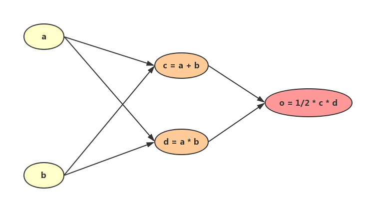
$\text{Figure 1: Simple Computational Graph}$

Our goal is to figure out how the changes of related variables affect the output, that is, to find out all the partial derivatives $\frac{\partial o}{\partial a}, \frac{\partial o}{\partial b}, \frac{\partial o}{\partial c}, \frac{\partial o}{\partial d}$ .

Let $a=2, b=3$ , we first move forward along the graph to compute the value of $c, d, o$ (the “feed-forward” process in neural network):

$\begin{align} & c = a + b = 2 + 3 = 5 \\ & d = ab = 2 \times 3 = 6 \\ & o = \frac{1}{2}cd = \frac{1}{2} \times 5 \times 6 = 15 \end{align}$

Next, we compute derivatives for each variable, using the “sum over paths” rule:

$\begin{align} & \frac{\partial o}{\partial a} = \frac{\partial o}{\partial c} \cdot \frac{\partial c}{\partial a} + \frac{\partial o}{\partial d} \cdot \frac{\partial d}{\partial a} = 10.5 \\ & \frac{\partial o}{\partial b} = \frac{\partial o}{\partial c} \cdot \frac{\partial c}{\partial b} + \frac{\partial o}{\partial d} \cdot \frac{\partial d}{\partial b} = 8 \\ & \frac{\partial o}{\partial c} = \frac{1}{2}d = 3 \\ & \frac{\partial o}{\partial d} = \frac{1}{2}c = 2.5 \\ \end{align}$

This is what we call “forward-mode differentiation”, in which we start from every variable and move forward to the output to compute the derivatives. Think about the computational paths we’ve gone through:

$\begin{align} & \frac{\partial o}{\partial a}: \left \{ \begin{array}{l} a \to c \to o \\ a \to d \to o \end{array} \right. \\ & \frac{\partial o}{\partial b}: \left \{ \begin{array}{l} b \to c \to o \\ b \to d \to o \end{array} \right. \\ & \frac{\partial o}{\partial c}: c \to o \\ & \frac{\partial o}{\partial d}: d \to o \end{align}$

We’ve repeated computing $\frac{\partial o}{\partial c}$ and $\frac{\partial o}{\partial d}$ for three times! As the number of variables increasing, the number of redundant computations would grow exponentially. Therefore, we need to improve the derivatives computations using a method like dynamic programming.

Here comes the “reverse-mode differentiation”. Instead of starting from each variable, we can start from the output and move backward to compute every derivative. First, we obtain:

$\frac{\partial o}{\partial o} = 1$

Next, we find that $o$ is the “parent” of $c$ and $d$ . Thus we get corresponding partial derivatives and stores them in memory:

$\begin{align} & \frac{\partial o}{\partial c} = \frac{1}{2}d = 3 \\ & \frac{\partial o}{\partial d} = \frac{1}{2}c = 2.5 \end{align}$

Finally, we find that both $c$ and $d$ are “parents” of $a$ and $b$ . We directly use $\frac{\partial o}{\partial c}$ and $\frac{\partial o}{\partial d}$ stored in memory to compute derivatives of $a$ and $b$ :

This is what we call “backpropagation”. In fact, it’s just a dynamic programming algorithm to compute the derivatives fast.

Backpropagation in Fully Connected Neural Network

$\text{Figure 2}$ shows a simple fully connected neural network structure:

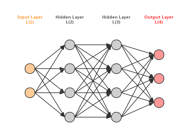
$\text{Figure 2: Simple Fully Connected Neural Network}$

We define following symbols:

Activation function: $F(x)$
Number of neural layers: $L$
Value of $j^{\text{th}}$ neuron in $l^{\text{th}}$ layer before activated: $z_j^l, 1 \le l \le L$
Value of $j^{\text{th}}$ neuron in $l^{\text{th}}$ layer after activated: $a_j^l = F(z_j^l), 1 \le l \le L$
Weight for the connection from $k^{\text{th}}$ neuron in $(l-1)^{\text{th}}$ to $j^{\text{th}}$ neuron in $l^{\text{th}}$ layer: $w^l_{jk}$
Bias for $j^{\text{th}}$ neuron in $l^{\text{th}}$ layer: $b^l_j$
Cost function: , where contains all the weights and biases that should be learned. There are two assumptions about from Nielsen’ book:
1. The cost function can be written as an average $J(\theta)=\frac{1}{n}\sum_x C_x$ , where $C_x$ denotes the cost of a single training example, $x$ .
2. The cost function can be written as a function of the outputs from the neural network: $J(\theta)=C(a^L)$
Error of $j^{\text{th}}$ neuron in $l^{\text{th}}$ layer (i.e, error of $z_j^l$ ): $\delta_j^l = \frac{\partial J(\theta)}{z_j^l}$ . This “error” measures how the changes of $z_j^l$ affect the cost function, meaning that $J(\theta)$ will change at a speed of $\delta_j^l$ when $z_j^l$ changes at a speed of $1$ . Hence, if a little change $\Delta z_j^l$ is added into $z_j^l$ to become $z_j^l + \Delta z_j^l$ , then $J(\theta)$ will change into $J(\theta) + \frac{\partial J(\theta)}{z_j^l} \Delta z_j^l = J(\theta) + \delta_j^l \Delta z_j^l$

Now suppose that we have a batch of training examples $X=\{(x^{(1)}, y^{(1)}), (x^{(2)}, y^{(2)}), ..., (x^{(n)}, y^{(n)})\}, x^{(i)} \in \mathbb R^2, y^{(i)} \in \mathbb R^3, 1 \le i \le n$ , which are fed into the network in $\text{Figure 2}$ to update all the weights $w_{jk}^l$ and biases $b_j^l$ using SGD. Hence, our goal is to find out all the gradients $\frac{\partial J(\theta)}{w_{jk}^l}$ and $\frac{\partial J(\theta)}{b_j^l}$ . First of all, for each training example $x^{(i)} = (x^{(i)}_1, x^{(i)}_2)$ with label $y^{(i)}$ , we run feed-forward to obtain its cost $C_i$ :

$\begin{align} & \text{Step 1:}~~~~ a^1 = \left [ \begin{array}{l} a_1^1 \\ a_2^1 \end{array} \right ] = z^1 = \left [ \begin{array}{l} z_1^1 \\ z_2^1 \end{array} \right ] = \left [ \begin{array}{l} x^{(i)}_1 \\ x^{(i)}_2 \end{array} \right ] \\ & \text{Step 2:}~~~~ z^2 = \left [ \begin{array}{l} w_{11}^2 \cdot a_1^1 + w_{12}^2 \cdot a_2^1 + b_1^2 \\ w_{21}^2 \cdot a_1^1 + w_{22}^2 \cdot a_2^1 + b_2^2 \\ w_{31}^2 \cdot a_1^1 + w_{32}^2 \cdot a_2^1 + b_3^2 \\ w_{41}^2 \cdot a_1^1 + w_{42}^2 \cdot a_2^1 + b_4^2 \end{array} \right ] = \left [ \begin{array}{l} z_1^2 \\ z_2^2 \\ z_3^2 \\ z_4^2 \\ \end{array} \right ], ~~ a^2 = F(z^2) = \left [ \begin{array}{l} F(z_1^2) \\ F(z_2^2) \\ F(z_3^2) \\ F(z_4^2) \end{array} \right ] = \left [ \begin{array}{l} a_1^2 \\ a_2^2 \\ a_3^2 \\ a_4^2 \\ \end{array} \right ] \\ & \text{Step 3:}~~~~ z^3 = \left [ \begin{array}{l} w_{11}^3 \cdot a_1^2 + w_{12}^3 \cdot a_2^2 + w_{13}^3 \cdot a_3^2 + w_{14}^3 \cdot a_4^2 + b_1^3 \\ w_{21}^3 \cdot a_1^2 + w_{22}^3 \cdot a_2^2 + w_{23}^3 \cdot a_3^2 + w_{24}^3 \cdot a_4^2 + b_2^3 \\ w_{31}^3 \cdot a_1^2 + w_{32}^3 \cdot a_2^2 + w_{33}^3 \cdot a_3^2 + w_{34}^3 \cdot a_4^2 + b_3^3 \\ w_{41}^3 \cdot a_1^2 + w_{42}^3 \cdot a_2^2 + w_{43}^3 \cdot a_3^2 + w_{44}^3 \cdot a_4^2 + b_4^3 \end{array} \right ] = \left [ \begin{array}{l} z_1^3 \\ z_2^3 \\ z_3^3 \\ z_4^3 \\ \end{array} \right ], ~~ a^3 = F(z^3) = \left [ \begin{array}{l} F(z_1^3) \\ F(z_2^3) \\ F(z_3^3) \\ F(z_4^3) \end{array} \right ] = \left [ \begin{array}{l} a_1^3 \\ a_2^3 \\ a_3^3 \\ a_4^3 \\ \end{array} \right ] \\ & \text{Step 4:}~~~~ z^4 = \left [ \begin{array}{l} w_{11}^4 \cdot a_1^3 + w_{12}^4 \cdot a_2^3 + w_{13}^4 \cdot a_3^3 + w_{14}^4 \cdot a_4^3 + b_1^4 \\ w_{21}^4 \cdot a_1^3 + w_{22}^4 \cdot a_2^3 + w_{23}^4 \cdot a_3^3 + w_{24}^4 \cdot a_4^3 + b_2^4 \\ w_{31}^4 \cdot a_1^3 + w_{32}^4 \cdot a_2^3 + w_{33}^4 \cdot a_3^3 + w_{34}^4 \cdot a_4^3 + b_3^4 \end{array} \right ] = \left [ \begin{array}{l} z_1^4 \\ z_2^4 \\ z_3^4 \end{array} \right ], ~~ a^4 = F(z^4) = \left [ \begin{array}{l} F(z_1^4) \\ F(z_2^4) \\ F(z_3^4) \end{array} \right ] = \left [ \begin{array}{l} a_1^4 \\ a_2^4 \\ a_3^4 \end{array} \right ] \\ & \text{Step 5:}~~~~ C_i = C(a^4, y^{(i)}) \end{align}$

After running the feed-forward for all training examples in $X$, we finally get $J(\theta) = \frac{1}{n}\sum_{i=1}^n C_i$. Unfortunately, we can not directly use $J(\theta)$ to compute all the gradients since different $x^{(i)}$ has different $a^4$. Instead, we compute the sample gradients for each training example $x^{(i)}$:

$\begin{align} & W_i = \frac{\partial C_i}{\partial w_{jk}^l} \\ & B_i = \frac{\partial C_i}{\partial b_j^l} \end{align}$

And then average all the sample gradients to obtain final gradients:

$\begin{align} & \frac{\partial J(\theta)}{\partial w_{jk}^l} = \frac{1}{n} \sum_{i=1}^{n} W_i \\ & \frac{\partial J(\theta)}{\partial b_j^l} = \frac{1}{n} \sum_{i=1}^{n} B_i \end{align}$

Now we begin to compute the sample gradients for a single training example $x^{(i)}$ . Before calculation, we should remember following 4 equations (let $L$ denotes the number of layers in a network, and $N^l$ denotes the number of neurons in layer $l$ ):

$\begin{align} & \text{Equation 1: } \frac{\partial C_i}{\partial w_{jk}^l} = \frac{\partial C_i}{\partial z_j^l} \cdot \frac{\partial z_j^l}{\partial w_{jk}^l} = \delta_j^l \cdot \frac{\partial (\sum_{p=1}^{N^{l-1}} w_{jp}^l a_p^{l-1} + b_j^l)}{\partial w_{jk}^l} = \delta_j^l \cdot a_k^{l-1}, ~~ 2 \le l \le L \\ & \text{Equation 2: } \frac{\partial C_i}{\partial b_j^l} = \frac{\partial C_i}{\partial z_j^l} \cdot \frac{\partial z_j^l}{\partial b_j^l} = \delta_j^l \cdot \frac{\partial (\sum_{p=1}^{N^{l-1}} w_{jp}^l a_p^{l-1} + b_j^l)}{\partial b_j^l} = \delta_j^l \cdot 1 = \delta_j^l, ~~ 2 \le l \le L \\ & \text{Equation 3: } \delta_j^l = \frac{\partial C_i}{\partial z_j^l} = \sum_{q=1}^{N^{l+1}} \frac{\partial C_i}{\partial z_q^{l+1}} \cdot \frac{\partial z_q^{l+1}}{\partial z_j^l} = \sum_{q=1}^{N^{l+1}} \delta_q^{l+1} \cdot \frac{\partial (\sum_{p=1}^{N^l} w_{qp}^{l+1} a_p^{l} + b_q^{l+1})}{\partial z_j^l} \\ & ~~~~~~~~~~~~~~~~~~~~~~~ = \sum_{q=1}^{N^{l+1}} \delta_q^{l+1} \cdot \frac{\partial [\sum_{p=1}^{N^l} w_{qp}^{l+1} F(z_p^{l}) + b_q^{l+1}]}{\partial z_j^l} = \sum_{q=1}^{N^{l+1}} \delta_q^{l+1} \cdot w_{qj}^{l+1}F'(z_j^{l}), ~~ 2 \le l \le L \\ & \text{Equation 4: } \delta_j^L = \frac{\partial C_i}{\partial z_j^L} = \frac{\partial C_i}{\partial a_j^L} \cdot \frac{\partial a_j^L}{\partial z_j^L} = \frac{\partial C_i}{\partial a_j^L} \cdot \frac{\partial F(z_j^L)}{\partial z_j^L} = \frac{\partial C_i}{\partial a_j^L} \cdot F'(z_j^L) \\ \end{align}$

In practice, we first compute $\text{Equation 4}$ , followed by applying $\text{Equation 3}$ on each layer to find out every $\delta_j^l$ , which is finally used to obtain our goals, $\text{Equation 1}$ and $\text{Equation 2}$ . Next, let’s begin our calculation:

$\begin{align} & \text{Step 1: } \delta^4 = \left [ \begin{array}{l} \frac{\partial C_i}{\partial a_1^4}F'(z_1^4) \\ \frac{\partial C_i}{\partial a_2^4}F'(z_2^4) \\ \frac{\partial C_i}{\partial a_3^4}F'(z_3^4) \end{array} \right ] = \left [ \begin{array}{l} \delta_1^4 \\ \delta_2^4 \\ \delta_3^4 \end{array} \right ] \\ & \text{Step 2: } \delta^3 = \left [ \begin{array}{l} F'(z_1^3)\cdot(\delta_1^4 w_{11}^4 + \delta_2^4 w_{21}^4 + \delta_3^4 w_{31}^4) \\ F'(z_2^3)\cdot(\delta_1^4 w_{12}^4 + \delta_2^4 w_{22}^4 + \delta_3^4 w_{32}^4) \\ F'(z_3^3)\cdot(\delta_1^4 w_{13}^4 + \delta_2^4 w_{23}^4 + \delta_3^4 w_{33}^4) \\ F'(z_4^3)\cdot(\delta_1^4 w_{14}^4 + \delta_2^4 w_{24}^4 + \delta_3^4 w_{34}^4) \end{array} \right ] = \left [ \begin{array}{l} \delta_1^3 \\ \delta_2^3 \\ \delta_3^3 \\ \delta_4^3 \end{array} \right ] \\ & \text{Step 3: } \delta^2 = \left [ \begin{array}{l} F'(z_1^2)\cdot(\delta_1^3 w_{11}^3 + \delta_2^3 w_{21}^3 + \delta_3^3 w_{31}^3 + \delta_4^3 w_{41}^3) \\ F'(z_2^2)\cdot(\delta_1^3 w_{12}^3 + \delta_2^3 w_{22}^3 + \delta_3^3 w_{32}^3 + \delta_4^3 w_{42}^3) \\ F'(z_3^2)\cdot(\delta_1^3 w_{13}^3 + \delta_2^3 w_{23}^3 + \delta_3^3 w_{33}^3 + \delta_4^3 w_{43}^3) \\ F'(z_4^2)\cdot(\delta_1^3 w_{14}^3 + \delta_2^3 w_{24}^3 + \delta_3^3 w_{34}^3 + \delta_4^3 w_{44}^3) \end{array} \right ] = \left [ \begin{array}{l} \delta_1^2 \\ \delta_2^2 \\ \delta_3^2 \\ \delta_4^2 \end{array} \right ] \\ & \text{Step 4: } \frac{\partial C_i}{\partial w^4} = \left [ \begin{array}{cccc} \delta_1^4 a_1^3 & \delta_1^4 a_2^3 & \delta_1^4 a_3^3 & \delta_1^4 a_4^3 \\ \delta_2^4 a_1^3 & \delta_2^4 a_2^3 & \delta_2^4 a_3^3 & \delta_2^4 a_4^3 \\ \delta_3^4 a_1^3 & \delta_3^4 a_2^3 & \delta_3^4 a_3^3 & \delta_3^4 a_4^3 \end{array} \right ], \frac{\partial C_i}{\partial w^3} = \left [ \begin{array}{cccc} \delta_1^3 a_1^2 & \delta_1^3 a_2^2 & \delta_1^3 a_3^2 & \delta_1^3 a_4^2 \\ \delta_2^3 a_1^2 & \delta_2^3 a_2^2 & \delta_2^3 a_3^2 & \delta_2^3 a_4^2 \\ \delta_3^3 a_1^2 & \delta_3^3 a_2^2 & \delta_3^3 a_3^2 & \delta_3^3 a_4^2 \\ \delta_4^3 a_1^2 & \delta_4^3 a_2^2 & \delta_4^3 a_3^2 & \delta_4^3 a_4^2 \end{array} \right ], \frac{\partial C_i}{\partial w^2} = \left [ \begin{array}{cc} \delta_1^2 a_1^1 & \delta_1^2 a_2^1 \\ \delta_2^2 a_1^1 & \delta_2^2 a_2^1 \\ \delta_3^2 a_1^1 & \delta_3^2 a_2^1 \\ \delta_4^2 a_1^1 & \delta_4^2 a_2^1 \end{array} \right ] \\ & \text{Step 5: } \frac{\partial C_i}{\partial b^4} = \left [ \begin{array}{l} \delta_1^4 \\ \delta_2^4 \\ \delta_3^4 \end{array} \right ], \frac{\partial C_i}{\partial b^3} = \left [ \begin{array}{l} \delta_1^3 \\ \delta_2^3 \\ \delta_3^3 \\ \delta_4^3 \end{array} \right ], \frac{\partial C_i}{\partial b^2} = \left [ \begin{array}{l} \delta_1^2 \\ \delta_2^2 \\ \delta_3^2 \\ \delta_4^2 \end{array} \right ] \end{align}$

Knowing formula of the activation function $F(x)$ and the cost function $J(\theta)$ , we can compute all the sample gradients we need. After averaging those sample gradients obtained through above 5 steps, we are able to find out every $\frac{\partial J(\theta)}{\partial w_{jk}^l}$ and $\frac{\partial J(\theta)}{\partial b_j^l}$ in a batch training data, and use SGD method to update the weights and biases.

Conclusion

Backpropagation is the key algorithm to build all kinds of deep learning models. Knowing how it works in dense neural network is the fundamental premise of understanding its role in nowadays advanced deep models, such as RNN, LSTM and CNN. I’ll continue to explain how it works in those models in later blogs.

How Does the Backpropagation Work (I)

Explain how backpropagation algorithm works in neural network

Introduction

Derivatives and Chain Rule

Derivatives on Simple Computational Graph

Backpropagation in Fully Connected Neural Network

Conclusion

References

CATALOG

FEATURED TAGS