Introduction
When talking about Convolutional Neural Network (CNN), we typically think of Computer Vision (CV) or Natural Language Processing (NLP). CNN was responsible for major breakthroughs in both Image Classification and Text Mining.
More recently, some researchers also start to apply CNNs on Multivariate Time Series Forecasting and get results better than traditional Autoregression model, such as Vector Autoregression (VAR). In this blog I’m going to explain how to apply CNNs on Multivariate Time Series and some related concepts.
Goal
Time Series Forecasting focuses on predicting the future values of variables we considered given their past, which amounts to expressing the expectation of future values as a function of the past observations:
Where $X_{i} = (x_{i}^1, x_{i}^2, …, x_{i}^n)$ is the vector of all concerned variables’ observations at time $i$. For example, we have following time series:
We consider , so on and so forth. Our goal is to figure out the values of , that is, the values of in the above table.
CNN Model
We design following CNN architecture:
1
Input -> Conv -> LeakyReLU -> Pool -> Conv -> LeakyReLU -> Dense
Next, we will go through the training process of our CNN step by step, using the example time series shown in $\text{Table 1}$. We’d like to figure out what CNN is doing with those data.
Part 1
$\text{Figure 1}$ depicts the first part Input -> Conv -> LeakyReLU -> Pool of our CNN:
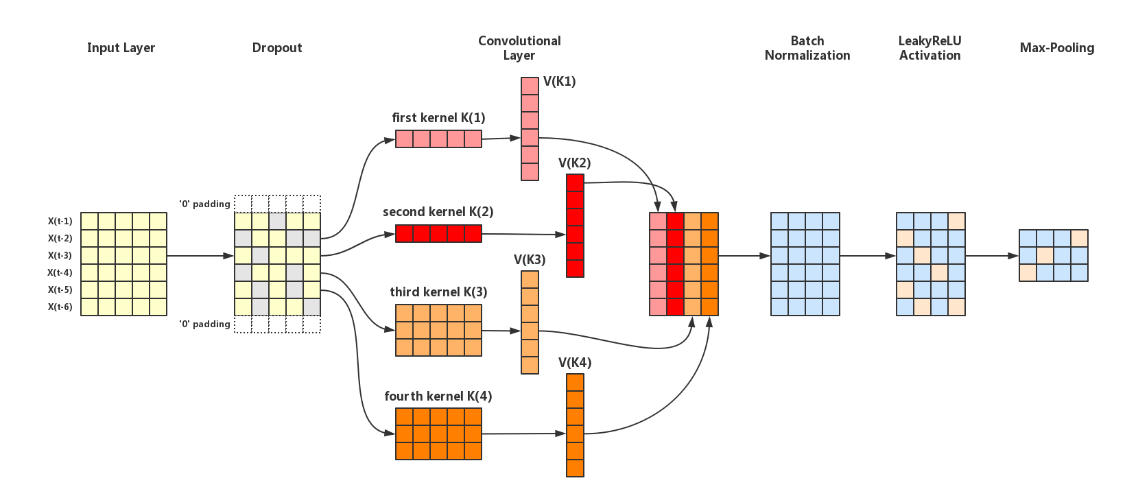
Input Layer & Dropout
For the Input Layer, we just input our data shown in $\text{Table 1}$. Before moving forward to Convolutional Layer, we apply Dropout with dropout_rate=0.5 on the input data. Assume that we finally get the following new dataset:
(For how to apply Dropout in CNN, please refer to Section 3.2 in Towards Dropout Training for Convolutional Neural Networks)
Convolutional Layer
For the Convolutional Layer, the convolution operation is quite similar to that in NLP. We design 2 kernels of shape(1, 5) (the first and second kernel in $\text{Figure 1}$) and 2 kernels of shape(3, 5) (the third and fourth kernel in $\text{Figure 1}$). For simplicity, we initilize all the kernels and their biases randomly, using the Numpy np.random.randn function to generate Gaussian distributions with mean $0$ and standard deviation $1$:
We just multiply the kernels of shape(1, 5) with $X_{i}$ in each row of $\text{Table 2}$ with element wise product, and add the biases to create elements of filtered vector (the $V_{K_{1}}$ ~ $V_{K_{4}}$ vectors in $\text{Figure 1}$):
Similiarly, we can obtain $V_{K_{2}}$ by convolving it and the second kernel:
Particularly, for the third and fourth kernel of shape(3, 5), we use the “SAME” pattern in Keras to apply $0$-padding on both end of the data in order to make sure the $V_{K_{3}}$ and $V_{K_{4}}$ we get have the same shape of $V_{K_{1}}$ and $V_{K_{2}}$. Unlike the first and second kernel, we should apply element wise product between every three rows (i.e.,$X_{i}, X_{i+1}, X_{i+2}$) and $K_{3}$ to obtain $V_{K_{3}}$:
Where $K_{3}^{(i)}$ denotes the $i$-th row of $K_{3}$ and $\sum{(V)}$ denotes the sum of all the elements in vector $V$. Similiarly, we get $V_{K_4}$:
Finally, concatenating all $V_{K_{i}}$ vectors generates the output of the Convolutional Layer:
Batch Normalization
Next, we move to Batch Normalization. Since we only have one data example rather than a “batch” of training dataset, we just use the mean and variance of each $V_{K_{i}}$ to normalize them and initilize $\gamma, \beta$ from Gaussian distributions with mean $0$ and standard deviation $1$:
(For how to apply Batch Normalization in CNN, please refer to Batch Normalization: Accelerating Deep Network Training by Reducing Internal Covariate Shift and Batch Normalization in Convolutional Neural Network)
Leaky ReLU Activation
Next, we should apply the Leaky ReLU function to each elements in $\text{BN_out}$:
Max Pooling
At the end of the first part, we apply Max Pooling on each $V_{K_{i}}$ of $\text{BN_out}$. Suppose the pooling_size=2, we get:
Part 2
$\text{Figure 2}$ depicts the second part Pool -> Conv -> LeakyReLU -> Dense of our CNN:
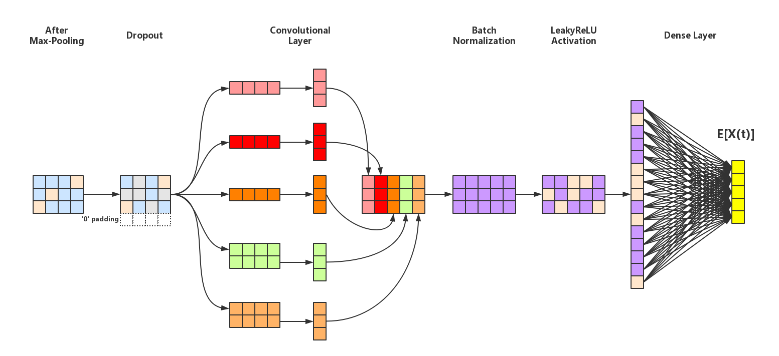
All the operations in Part 2 are similar to Part 1. After the Dense Layer, we’ll eventually get the $\mathbb{E}[X_{t}]$ which will be used to calculate the loss function during training.
Conclusion
We just have gone through the whole training process of one time series sample in CNN, illustrating the concepts of Dropout, Convolution, Batch Normalization and Max Pooling. I hope this process could be helpful to understand how the CNN works with Multivariate Time Series Forecasting. In the next blog, I’ll train a CNN model for Multivariate Time Series Forecasting using Tensorflow.