Learn the Neural Networks with Tensorflow (I)

Introduction

Thanks to Michael Nielsen’s book Neural Networks and Deep Learning and TensorFlow Tutorial and Examples for Beginners with Latest APIs, I’ve spent an easier life on learning neural networks. In order to put what I’ve learned into practice, I decide to repeat the experiments in the book using Tensorflow, a powerful tool for machine learning. This blog shows the result of the first experiment, which builds a simple fully-connected neural network to classify MNIST handwritten digits.

Data Preprocessing

We use the MNIST data provided in Nielsen’s code and his function load_data() to load the trainning, validation and test data respectively.

import pickle
import gzip

def load_data():
    """Return the MNIST data as a tuple containing the training data,
    the validation data, and the test data.

    The ``training_data`` is returned as a tuple with two entries.
    The first entry contains the actual training images.  This is a
    numpy ndarray with 50,000 entries.  Each entry is, in turn, a
    numpy ndarray with 784 values, representing the 28 * 28 = 784
    pixels in a single MNIST image.

    The second entry in the ``training_data`` tuple is a numpy ndarray
    containing 50,000 entries.  Those entries are just the digit
    values (0...9) for the corresponding images contained in the first
    entry of the tuple.

    The ``validation_data`` and ``test_data`` are similar, except
    each contains only 10,000 images.

    This is a nice data format, but for use in neural networks it's
    helpful to modify the format of the ``training_data`` a little.
    That's done in the wrapper function ``load_data_wrapper()``, see
    below.
    """
    f = gzip.open('./data/mnist.pkl.gz', 'rb')
    loader = pickle._Unpickler(f)
    loader.encoding = 'latin1'
    training_data, validation_data, test_data = loader.load()
    f.close()
    return (training_data, validation_data, test_data)

Since we should apply Stochastic Gradient Descent (SGD) method to train our neural network, it’s necessary to randomly shuffle our trainning data in order to select batch data in every epoch of training. It’s helpful to shuffle trainning data first and then read them in order, which improves cache hits and speeds up learning process.

import numpy as np

# randomly shuffle the training data
def random_shuffle(data_features, data_labels):
    indices = np.random.permutation(data_features.shape[0])
    X = data_features[indices]
    Y = data_labels[indices]
    return X, Y

Let’s read our data and see what we get:

print ('reading data...')
# read the data from file
training_data, validation_data, test_data = load_data()

# get the trainning data
train_X = training_data[0]
train_Y = training_data[1]
# get the test data
test_X = test_data[0]
test_Y = test_data[1]

print ('training data features: %s, trainning data labels: %s' % (train_X.shape, train_Y.shape))
print ('test data features: %s, test data labels: %s' % (test_X.shape, test_Y.shape))

reading data...
training data features: (50000, 784), trainning data labels: (50000,)
test data features: (10000, 784), test data labels: (10000,)

We see that there are 50000 samples in the trainning data and 10000 samples in the test data. Note that we don’t use the validation data here, which helps figure out how to set hyper-parameters of our neural network later.

Neural Network

We use a three-layer neural network with (784, 30, 10) neurons to recognize the digits (0-9, 10 classes):

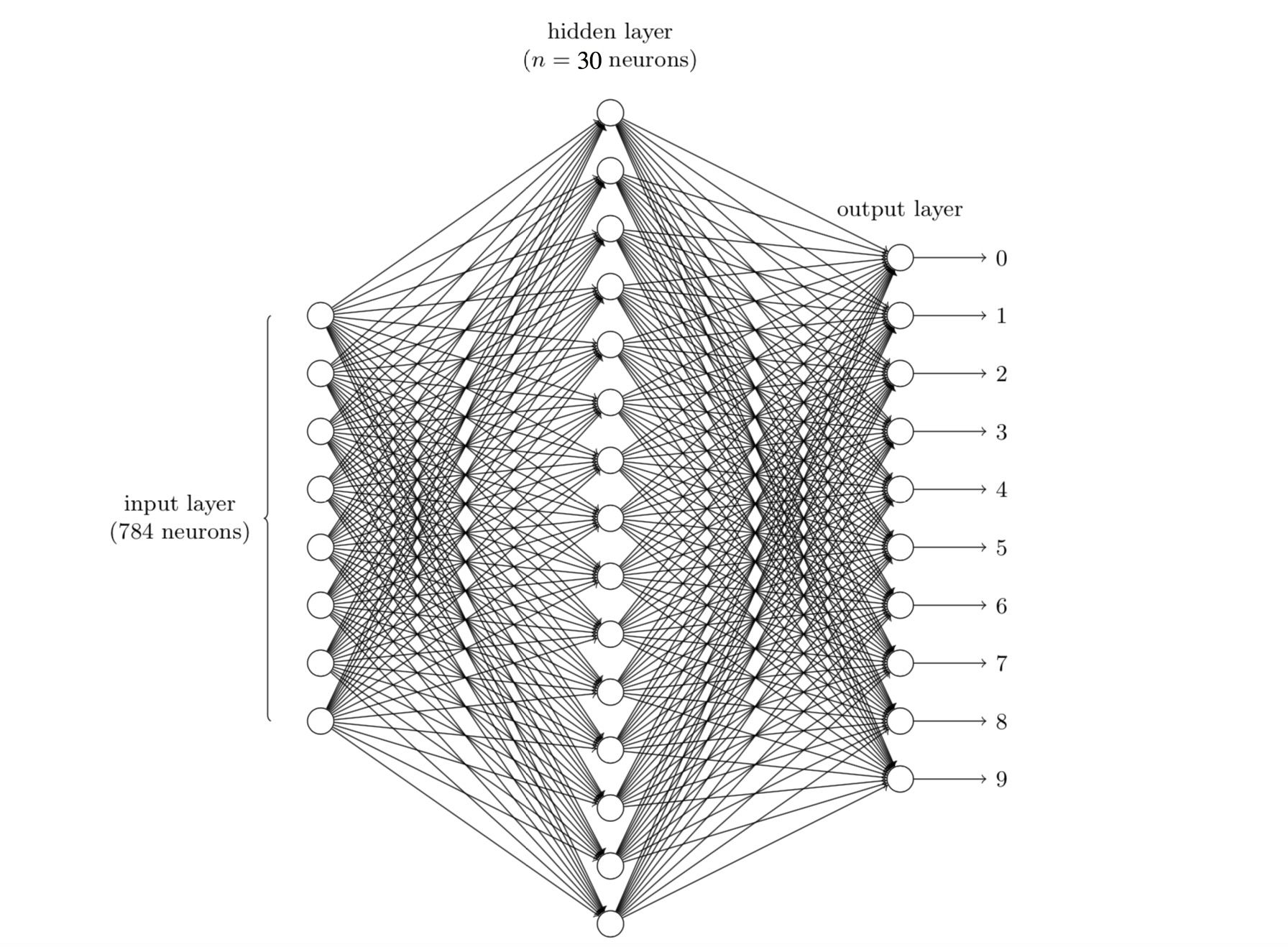
We have 10 neurons as output to recognize the digit, meaning that a digit’s label should be represented as a 10-dimension vector. For example, if the label of the $i$-th sample $x^{(i)}$ is $4$ , we represent its label as $y^{(i)} = (0, 0, 0, 0, 1, 0, 0, 0, 0, 0)$ ; if the label of the $i$-th sample $x^{(i)}$ is $9$, we represent its label as $y^{(i)} = (0, 0, 0, 0, 0, 0, 0, 0, 0, 1)$ , so on and so forth. Therefore, we extend the label of each digit to the shape of (10,). Consequently, the shape of Y and test_Y would be extended to (50000, 10) and (10000, 10), respectively.

# extend the data from shape(data.shape[0],) to shape(data.shape[0], dim)
def to_vector(data, dim):
    data_vector = np.zeros([data.shape[0], dim], dtype=np.float64)
    for i in range(data.shape[0]):
        index = data[i]
        data_vector[i][index] = 1.0
    return data_vector

trainY_vector = to_vector(train_Y, 10)
testY_vector = to_vector(test_Y, 10)
print ('training data shape: ', trainY_vector.shape)
print ('test data shape: ', testY_vector.shape)

training data shape:  (50000, 10)
test data shape:  (10000, 10)

The trainning configuration and hyper-parameters are set as follows:

activation function: $\sigma (z) = \frac{1}{1 + e^{-z}}$
cost function: $J(\theta) = \frac{1}{2N} \sum_{i = 1}^{N} ||y^{(i)} - h(x^{(i)})||^2 $, where $N$ is the total number of training inputs, $y^{(i)}$ is the vector of $i$-th sample’s label, $h(x^{(i)})$ is the vector of $i$-th sample’s prediction label. $\theta$ contains the weights $w$ and the biases $b$ of neurons.
training epochs: $30$
mini-batch size: $10$
learning rate: $\eta = 3.0$

Construct the Network with Raw Tensorflow

Next, let’s design our neural network step by step using Tensorflow:

import tensorflow as tf

# set the hyper-parameters
epochs = 30
mini_batch_size = 10
learning_rate = 3.0
display_epoch = 5     # display the learning state every 5 epochs

# set the network parameters
input_neurons_num = 784
hidden_1_neurons_num = 30
output_neurons_num = 10

# define the parameter to be fed 
t_X = tf.placeholder(tf.float64, [None, input_neurons_num])
t_Y = tf.placeholder(tf.float64, [None, output_neurons_num])

# define the weights and biases, generated from Gaussian distributions with mean 0 and standard deviation 1
weights = {
    'input_to_h1': tf.Variable(tf.random_normal([input_neurons_num, hidden_1_neurons_num], mean=0.0, stddev=1.0, dtype=tf.float64)),
    'h1_to_output': tf.Variable(tf.random_normal([hidden_1_neurons_num, output_neurons_num], mean=0.0, stddev=1.0, dtype=tf.float64))
}
biases = {
    'h1': tf.Variable(tf.random_normal([hidden_1_neurons_num], mean=0.0, stddev=1.0, dtype=tf.float64)),
    'output': tf.Variable(tf.random_normal([output_neurons_num], mean=0.0, stddev=1.0, dtype=tf.float64))
}

# feedforward process
def predict(x):
    """
    predict the label of trainning data x through the network
    :param x shape[None, input_neurons_num] the trainning data
    :return output_layer shape[None, output_neurons_num] the output vector of training data
    """
    h1_layer = tf.sigmoid(tf.add(tf.matmul(x, weights['input_to_h1']), biases['h1']))
    output_layer = tf.sigmoid(tf.add(tf.matmul(h1_layer, weights['h1_to_output']), biases['output']))
    return output_layer

# construct the model
logit = predict(t_X)

# set the cost function and SGD optimizer
cost_op = tf.reduce_sum(((t_Y - logit) ** 2))  / (2 * mini_batch_size)
optimizer = tf.train.GradientDescentOptimizer(learning_rate=learning_rate)
train_op = optimizer.minimize(cost_op)

# evaluate the model with accuracy
correct_num = tf.equal(tf.argmax(logit, 1), tf.argmax(t_Y, 1))
accuracy = tf.reduce_mean(tf.cast(correct_num, tf.float32))

# Initialize the variables (i.e. assign their default value)
init = tf.global_variables_initializer()

Finally, we train the model and evaluate the result. In order to better observe the learning process, we display the accuracy of the test data every 5 epochs:

with tf.Session() as sess:
    # Run the initializer
    sess.run(init)
    # for each epoch, use mini-batch SGD to train the weights and biases
    for current_epoch in range(0, epochs):
        # randomly shuffle the training data first
        X, Y = random_shuffle(training_data[0], training_data[1])
        # extend the label
        Y_vector = to_vector(Y, 10)
        # run SGD
        for i in range(0, X.shape[0], mini_batch_size):
            batch_x = X[i:(i+mini_batch_size)]
            batch_y = Y_vector[i:(i+mini_batch_size)]
            sess.run(train_op, feed_dict={t_X: batch_x, t_Y: batch_y})
        
        # print the accuracy every 5 epochs
        if (current_epoch+1) % display_epoch == 0 or current_epoch == 0:
            # Calculate accuracy for MNIST test images under current epoch
            print "Epoch %i, Testing Accuracy: %.4f" % (current_epoch+1, sess.run(accuracy, feed_dict={t_X: test_X, t_Y: testY_vector}))
            
    print "Optimization Finished!"

Epoch 1, Testing Accuracy: 0.9053
Epoch 5, Testing Accuracy: 0.9356
Epoch 10, Testing Accuracy: 0.9460
Epoch 15, Testing Accuracy: 0.9494
Epoch 20, Testing Accuracy: 0.9485
Epoch 25, Testing Accuracy: 0.9525
Epoch 30, Testing Accuracy: 0.9510
Optimization Finished!

The finally accuracy is $95.10\%$, a satisfactory result for such a simple network. Also, the accuracy is close to that in Nielsen’s book.

Construct the Network with `layers` API

The process of constructing our network using raw Tensorflow is quiet tedious and easy to cause bugs, in which we define the weights and biases, mutiply the weights and add the biases manually. Fortunately, Tensorflow provides more powerful API to simplify our work, one of which is the layers API. Let’s make our life easier!

# set the hyper-parameters
epochs = 30
mini_batch_size = 10
learning_rate = 3.0
display_epoch = 5     # display the learning state every 5 epochs

# set the network parameters
input_neurons_num = 784
hidden_1_neurons_num = 30
output_neurons_num = 10

# define the parameter to be fed 
t_X = tf.placeholder(tf.float64, [None, input_neurons_num])
t_Y = tf.placeholder(tf.float64, [None, output_neurons_num])

# feedforward process
def predict_with_layer(x):
    """
    predict the label of trainning data x through the network using tf.layers
    :param x shape[None, input_neurons_num] the trainning data
    :return output_layer shape[None, output_neurons_num] the output vector of training data
    """
    h1_layer = tf.layers.dense(x, 
                               hidden_1_neurons_num, 
                               activation=tf.sigmoid, 
                               kernel_initializer=tf.random_normal_initializer(mean=0.0, stddev=1.0, dtype=tf.float64),
                               bias_initializer=tf.random_normal_initializer(mean=0.0, stddev=1.0, dtype=tf.float64))
    output_layer = tf.layers.dense(h1_layer, 
                                   output_neurons_num,
                                   activation=tf.sigmoid,
                                   kernel_initializer=tf.random_normal_initializer(mean=0.0, stddev=1.0, dtype=tf.float64),
                                   bias_initializer=tf.random_normal_initializer(mean=0.0, stddev=1.0, dtype=tf.float64))
    return output_layer

# construct the model
logit = predict_with_layer(t_X)

# set the cost function and SGD optimizer
cost_op = tf.reduce_sum(((t_Y - logit) ** 2))  / (2 * mini_batch_size)
optimizer = tf.train.GradientDescentOptimizer(learning_rate=learning_rate)
train_op = optimizer.minimize(cost_op)

# evaluate the model with accuracy
correct_num = tf.equal(tf.argmax(logit, 1), tf.argmax(t_Y, 1))
accuracy = tf.reduce_mean(tf.cast(correct_num, tf.float32))

# Initialize the variables (i.e. assign their default value)
init = tf.global_variables_initializer()

Finally, we train our network and evaluate the model with test data. In order to better observe the learning process, we display the accuracy of the test data every 5 epochs:

with tf.Session() as sess:
    # Run the initializer
    sess.run(init)
    # for each epoch, use mini-batch SGD to train the weights and biases
    for current_epoch in range(0, epochs):
        # randomly shuffle the training data first
        X, Y = random_shuffle(training_data[0], training_data[1])
        # extend the label
        Y_vector = to_vector(Y, 10)
        # run SGD
        for i in range(0, X.shape[0], mini_batch_size):
            batch_x = X[i:(i+mini_batch_size)]
            batch_y = Y_vector[i:(i+mini_batch_size)]
            sess.run(train_op, feed_dict={t_X: batch_x, t_Y: batch_y})
        
        # print the accuracy every 5 epochs
        if (current_epoch+1) % display_epoch == 0 or current_epoch == 0:
            # Calculate accuracy for MNIST test images under current epoch
            print "Epoch %i, Testing Accuracy: %.4f" % (current_epoch+1, sess.run(accuracy, feed_dict={t_X: test_X, t_Y: testY_vector}))
            
    print "Optimization Finished!"

Epoch 1, Testing Accuracy: 0.8244
Epoch 5, Testing Accuracy: 0.9294
Epoch 10, Testing Accuracy: 0.9373
Epoch 15, Testing Accuracy: 0.9426
Epoch 20, Testing Accuracy: 0.9429
Epoch 25, Testing Accuracy: 0.9463
Epoch 30, Testing Accuracy: 0.9416
Optimization Finished!

We see the final accuracy is $94.16\%$, close to the result we first got. The random initilization of weights and biases might affect the accuracy slightly.

Train the Network with `estimator` API

Sometimes we want to see the change of the cost and the accuracy during both training and testing processes, followed by comparison and analysis between the two process. Instead of plotting the curves manually, we can turn to estimator API provided by Tensorflow. tf.estimator.Estimator object stores necessary information of each step while running and we can view the trend graphs of loss and accuracy later in TensorBoard. Since the estimator API will store a lot of information during each step, we should decrease epochs to 1 in order to speed up the training. Note that the steps and epochs parameters are totally different concepts. steps is the number of times the weights and biases of our network needs to be updated, while epoch refers to the number of times the network goes through the entire training dataset. For example, with mini_batch_size = 10, the weights and biases will be updated after our network goes through 10 trainning samples, meaning that our network has finished one step. There are total 50000 trainning sample, leading to $\frac{50000}{10} = 5000$ steps before our network has gone through the entire dataset for one time (i.e. one epoch). In this case we have $1 \text{ epoch} = 5000 \text{ steps}$. We can define either steps or epochs in estimator API to control the trainning times. Here we just set epochs = 1 and leave steps unset.

import tensorflow as tf

# set the hyper-parameters
epochs = 1
mini_batch_size = 10
learning_rate = 3.0
num_steps = None

# set the network parameters
input_neurons_num = 784
hidden_1_neurons_num = 30
output_neurons_num = 10

# translate the training and test data into dictionary in order to feed Estimator's input
train_X_es = {}
test_X_es = {}
feature_columns = []
for i in range(train_X.shape[1]):
    train_X_es['pixel_' + str(i)] = train_X[:, i]
    test_X_es['pixel_' + str(i)] = test_X[:, i]
    feature_columns.append(tf.feature_column.numeric_column(key='pixel_' + str(i)))
    
# feedforward process
def predict_with_layer(x):
    """
    predict the label of trainning data x through the network using tf.layers
    :param x shape[None, input_neurons_num] the trainning data
    :return output_layer shape[None, output_neurons_num] the output vector of training data
    """
    input_layer = tf.feature_column.input_layer(x, feature_columns)
    h1_layer = tf.layers.dense(input_layer,
                              hidden_1_neurons_num,
                              activation=tf.sigmoid,
                              kernel_initializer=tf.random_normal_initializer(mean=0.0, stddev=1.0, dtype=tf.float64),
                              bias_initializer=tf.random_normal_initializer(mean=0.0, stddev=1.0, dtype=tf.float64))
    output_layer = tf.layers.dense(h1_layer, 
                                   output_neurons_num,
                                   activation=tf.sigmoid,
                                   kernel_initializer=tf.random_normal_initializer(mean=0.0, stddev=1.0, dtype=tf.float64),
                                   bias_initializer=tf.random_normal_initializer(mean=0.0, stddev=1.0, dtype=tf.float64))
    return output_layer

# define the training and test input function to Estimator
train_input_fn = tf.estimator.inputs.numpy_input_fn(
    x=train_X_es, y=trainY_vector, batch_size=mini_batch_size, num_epochs=epochs, shuffle=True)
test_input_fn = tf.estimator.inputs.numpy_input_fn(
    x=test_X_es, y=testY_vector, shuffle=False)

# define the model function (following tf.Estimator template)
def model_fn(features, labels, mode):
    """
    :param features dict of array objects representing features value
    :param labels list of labels of each sample
    :param mode Estimator mode
    """
    # predict
    logits = predict_with_layer(features)
    
    # results
    pred_classes = tf.argmax(logits, axis=1)
    real_classes = tf.argmax(labels, axis=1)
    
    # if prediction mode, only return the results
    if mode == tf.estimator.ModeKeys.PREDICT:
        return tf.estimator.EstimatorSpec(mode, predictions=logits)
    
    # define cost and optimizer
    cost_op = tf.reduce_sum((labels - tf.cast(logits, dtype=tf.float64)) ** 2.0) / (2.0 * mini_batch_size)
    optimizer = tf.train.GradientDescentOptimizer(learning_rate=learning_rate)
    train_op = optimizer.minimize(cost_op, global_step=tf.train.get_global_step())
    
    # Evaluate the accuracy of the model
    acc_op = tf.metrics.accuracy(labels=real_classes, predictions=pred_classes)
    
    # show the accuracy change in the Tensorboard
    tf.summary.scalar('accuracy', acc_op[1])
    
    # tf.Estimators requires to return a EstimatorSpec that specify the different ops for training, evaluating, testing
    estim_specs = tf.estimator.EstimatorSpec(
      mode=mode,
      predictions=logits,
      loss=cost_op,
      train_op=train_op,
      eval_metric_ops={'accuracy': acc_op})
    
    return estim_specs

# build the Estimator
# the model_dir parameters refers to the directory that stored information for TensorBoard
model = tf.estimator.Estimator(model_fn, model_dir='./train_process/')

# train the Model
model.train(train_input_fn, steps=num_steps)

INFO:tensorflow:Using default config.

......

INFO:tensorflow:loss = 1.4296132314955696, step = 1
INFO:tensorflow:global_step/sec: 19.2492
INFO:tensorflow:loss = 0.4606772967635693, step = 101 (5.198 sec)
INFO:tensorflow:global_step/sec: 33.211
INFO:tensorflow:loss = 0.30009716419059806, step = 201 (3.009 sec)
INFO:tensorflow:global_step/sec: 33.4108
INFO:tensorflow:loss = 0.31261175006482733, step = 301 (2.991 sec)
INFO:tensorflow:global_step/sec: 34.0583
INFO:tensorflow:loss = 0.34764309040642677, step = 401 (2.937 sec)
INFO:tensorflow:global_step/sec: 32.5743
INFO:tensorflow:loss = 0.17760775757722494, step = 501 (3.073 sec)
INFO:tensorflow:global_step/sec: 31.6378
INFO:tensorflow:loss = 0.044561736962616214, step = 601 (3.157 sec)
INFO:tensorflow:global_step/sec: 32.4939
INFO:tensorflow:loss = 0.1688654795899642, step = 701 (3.076 sec)
INFO:tensorflow:global_step/sec: 30.3249
INFO:tensorflow:loss = 0.2513630772900814, step = 801 (3.302 sec)
INFO:tensorflow:global_step/sec: 31.5121
INFO:tensorflow:loss = 0.07362611853771173, step = 901 (3.181 sec)
INFO:tensorflow:global_step/sec: 34.6231
INFO:tensorflow:loss = 0.16010246881727905, step = 1001 (2.880 sec)

......

INFO:tensorflow:global_step/sec: 33.3311
INFO:tensorflow:loss = 0.1641046707857765, step = 4001 (3.006 sec)
INFO:tensorflow:global_step/sec: 32.428
INFO:tensorflow:loss = 0.009008384208704662, step = 4101 (3.079 sec)
INFO:tensorflow:global_step/sec: 31.4536
INFO:tensorflow:loss = 0.1403828176797829, step = 4201 (3.177 sec)
INFO:tensorflow:global_step/sec: 33.4421
INFO:tensorflow:loss = 0.11668906005834107, step = 4301 (2.990 sec)
INFO:tensorflow:global_step/sec: 33.1435
INFO:tensorflow:loss = 0.0013682651296430556, step = 4401 (3.020 sec)
INFO:tensorflow:global_step/sec: 32.6878
INFO:tensorflow:loss = 0.0635278685221181, step = 4501 (3.056 sec)
INFO:tensorflow:global_step/sec: 33.6172
INFO:tensorflow:loss = 0.02669870323195274, step = 4601 (2.975 sec)
INFO:tensorflow:global_step/sec: 35.1905
INFO:tensorflow:loss = 0.029559657127118055, step = 4701 (2.851 sec)
INFO:tensorflow:global_step/sec: 32.3153
INFO:tensorflow:loss = 0.13364987549250787, step = 4801 (3.085 sec)
INFO:tensorflow:global_step/sec: 32.2163
INFO:tensorflow:loss = 0.08868286066716438, step = 4901 (3.104 sec)
INFO:tensorflow:Saving checkpoints for 5000 into ./train_process/model.ckpt.
INFO:tensorflow:Loss for final step: 0.08273879671613951.

# evaluate the Model
model.evaluate(test_input_fn)

INFO:tensorflow:Calling model_fn.
INFO:tensorflow:Done calling model_fn.
INFO:tensorflow:Starting evaluation at 2018-11-08-02:40:39
INFO:tensorflow:Graph was finalized.
INFO:tensorflow:Restoring parameters from ./train_process/model.ckpt-5000
INFO:tensorflow:Running local_init_op.
INFO:tensorflow:Done running local_init_op.
INFO:tensorflow:Finished evaluation at 2018-11-08-02:40:49
INFO:tensorflow:Saving dict for global step 5000: accuracy = 0.9126, global_step = 5000, loss = 0.9034075
INFO:tensorflow:Saving 'checkpoint_path' summary for global step 5000: ./train_process/model.ckpt-5000



{'accuracy': 0.9126, 'loss': 0.9034075, 'global_step': 5000}

It seems that the performance of the network drops around $4\%$ due to the decrease of training epochs. However, the the network still has a high accuracy $91.26\%$, because the SGD method made the weights and biases updated enough times in, though, only one epoch. Next, we go to the directory referred by model_dir and type following instruction:

tensorboard --logdir=$(your_model_dir)

Then open http://localhost:6006 in your web browser, you can see the trends of accuracy and loss of training:

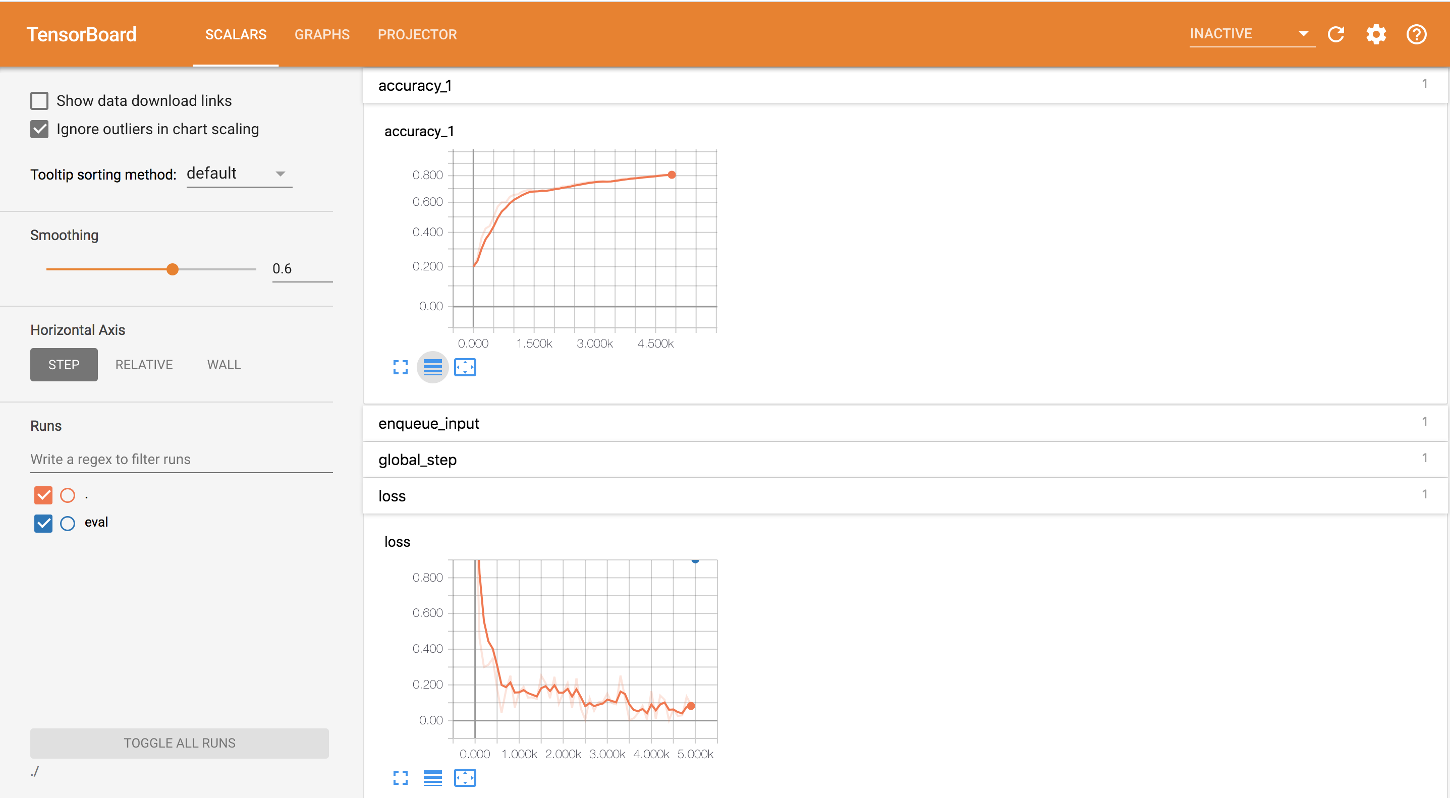
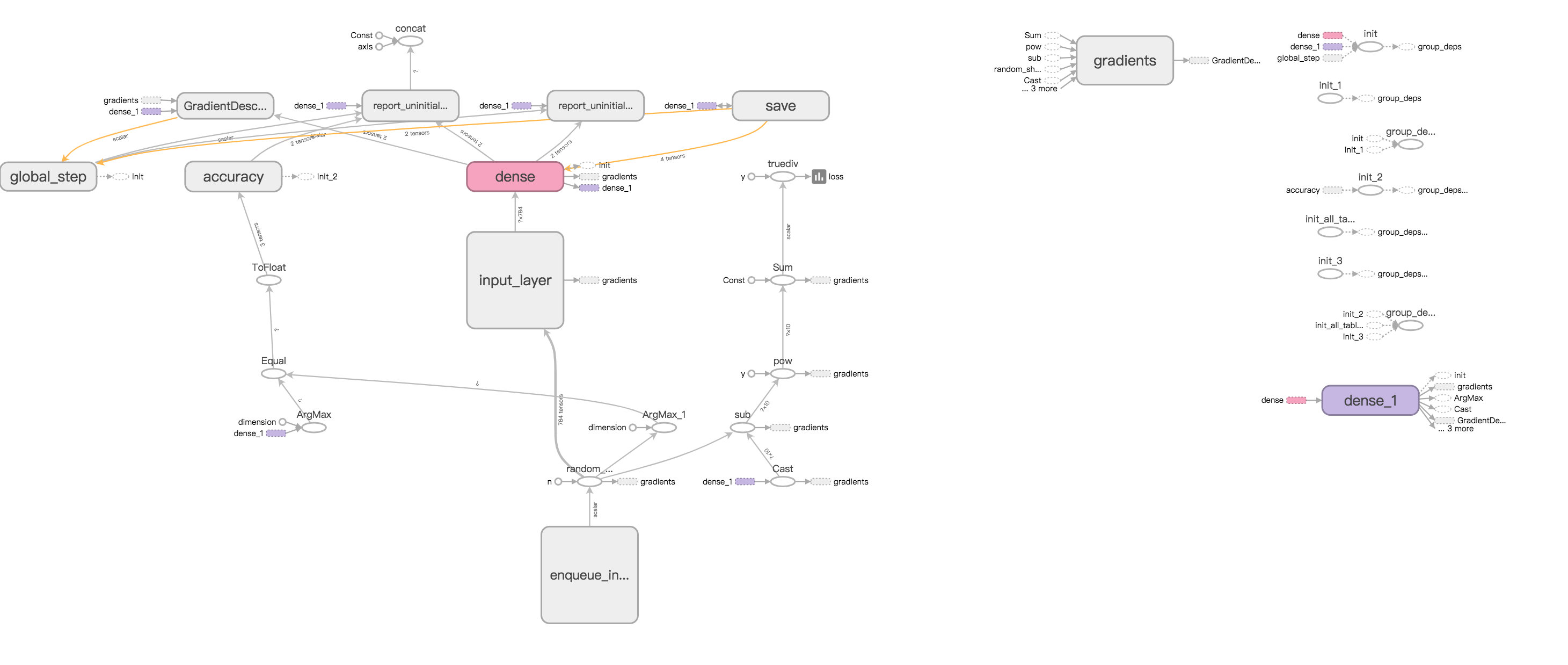
You can also view the network structure by click the GRAPHS option:

Conclusion

We’ve repeated the first experiment in Nielsen’s book and got a satisfactory result. I’ll continue to repeat other experiments using Tensorflow in later blogs, exploring the relative factors that could affect neural network’s training speed and accuracy, such as the learning rate, the mini-batch size, the regularization, the network structure, etc.

Learn the Neural Networks with Tensorflow (I)

A summary of using Tensorflow to train Neural Networks

Introduction

Data Preprocessing

Neural Network

Construct the Network with Raw Tensorflow

Construct the Network with `layers` API

Train the Network with `estimator` API

Conclusion

CATALOG

FEATURED TAGS

Introduction

Data Preprocessing

Neural Network

Construct the Network with Raw Tensorflow

Construct the Network with layers API

Train the Network with estimator API

Conclusion

CATALOG

FEATURED TAGS

Construct the Network with `layers` API

Train the Network with `estimator` API